Overview
This lesson implements some really important training techniques today, all using callbacks:
- MixUp: a data augmentation technique that dramatically improves results, particularly when you have less data, or can train for a longer time.
- Label smoothing: which works particularly well with MixUp, and significantly improves results when you have noisy labels
- Mixed precision training: which trains models around 3x faster in many situations.
- It also implement XResNet: which is a tweaked version of the classic resnet architecture that provides substantial improvements. And, even more important, the development of it provides great insights into what makes an architecture work well.
- Finally, the lesson show how to implement ULMFiT from scratch, including building an LSTM RNN, and looking at the various steps necessary to process natural language data to allow it to be passed to a neural network.
Even Better Image Training: Mixup/Label Smoothing
MixUp
(Notebook: 10b_mixup_label_smoothing.ipynb)
It’s quite possible that we don’t need much data augmentation for images anymore. FastAI’s experiments with a data augmentation called Mixup, they found that they could remove most other data augmentation and get amazingly good results. It’s really simple to do and you can also train with MixUp for a really long time and get really good results.
- MixUp comes from the paper: mixup: Beyond Empirical Risk Minimization [2017]. This is quite an easy reading paper.
- MixUp was shown to be a very effective training technique in the paper: Bag of Tricks for Image Classification with Convolutional Neural Networks [2019]. (This lesson will refer back to this paper a lot so it’s also worth reading fully.)
Here is the table of results for the different training tricks tried in that paper:
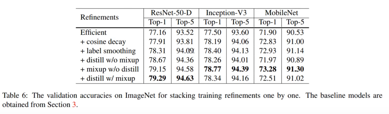
(NB with MixUp they ran for more epochs)
What is MixUp? We are going to take two different images and we are going to combine them. How? By simply making a convex combination of the two. So you do 30% of one image and 70% of the other image:
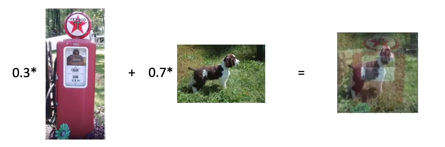
You also have to do MixUp to the labels. So rather than being a one-hot encoded target, your target would become something like:
y = [0.3 (gas pump), 0.7 (dog)]
When we are generating these mixed up training examples on the fly we we need to pick how much of each image we will use. Let’s define a mixing proportion, $\lambda$, so our mixed image will be $\lambda x_i + (1-\lambda) x_j$ . We will pick the $\lambda$ randomly each time, however we don’t want to just naively generate this from a uniform distribution. In the MixUp paper they explore how the mixing parameter affects performance and they get this plot (higher is worse):
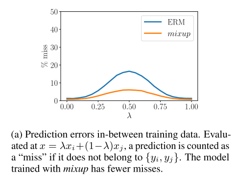
For good values we need to sample from a distribution that is more likely to pick numbers near 0 or near 1. A distribution that looks like this is the beta distribution.
It is one of the weirder distributions and it’s not very intuitive from its formula, but the shape of it looks like this for two different values of the parameters $\alpha$:
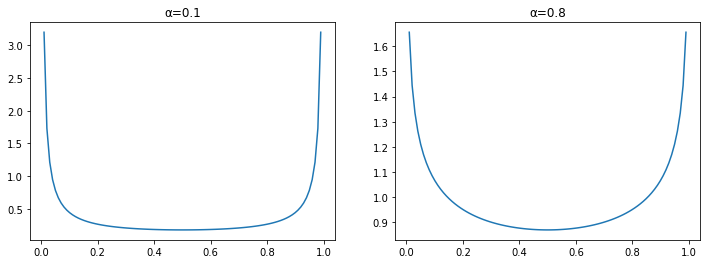
The Beta distribution tends to generate number at the edges. If you compare that to the plot of prediction errors above you can see they are inverses of each other.
(Aside: this SO post about the intuition behind the Beta distribution is quite interesting).
Let’s look at the implementation of MixUp…
Original MixUp Algorithm: In the original article, the authors suggested three things:
- Create two separate dataloaders and draw a batch from each at every iteration to mix them up
- Draw a $\lambda$ value following a beta distribution with a parameter $\alpha$ (0.4 is suggested in their article)
- Mix up the two batches with the same value $\lambda$.
- Use one-hot encoded targets
While the approach above works very well, it’s not the fastest way we can do this. The main point that slows down this process is wanting two different batches at every iteration (which means loading twice the amount of images and applying to them the other data augmentation function). To avoid this slow down, we can be a little smarter and mixup a batch with a shuffled version of itself (this way the mixed up images are still different). This was a trick suggested in the MixUp paper.
FastAI MixUp Algorithm: FastAI employs a few tricks to improve it:
-
Create a single dataloader and draw a single batch, $X$, with labels $y$ from which we can create mixed up images by shuffling this batch.
-
For each item in the batch pick a generate a vector of $\lambda$ values (Beta distribution with $\alpha=0.4$). To avoid potential duplicate mixups fix $\lambda$ values with:
λ = max(λ, 1-λ) -
Create a random permutation of the batch $X’$ and labels $y’$.
-
Return the linear combination of the original batch and the random permutation: $\lambda X + (1-\lambda) X’$. Likewise with the labels: $\lambda y + (1-\lambda)y’$.
The first trick is picking a different $\lambda$ for every image in the batch because fastai found that doing so made the network converge faster.
The second trick is using a single batch and shuffling it for MixUp instead of loading two batches. However, this strategy can create duplicates. Let’s say the batch has two images, we shuffle the batch and first mix Image0 with Image1 with $\lambda_1=0.1$, and then mix Image1 and Image0 with $\lambda=0.9$:
image0 * 0.1 + shuffle0 * (1-0.1) = image0 * 0.1 + image1 * 0.9
image1 * 0.9 + shuffle1 * (1-0.9) = image1 * 0.9 + image0 * 0.1
These will be the same. Of course, we have to be a bit unlucky but in practice, they saw there was a drop in accuracy by using this without removing those near-duplicates. To avoid them, the tricks is to replace the vector of parameters we drew by:
λ = max(λ, 1-λ)
The beta distribution with the two parameters equal is symmetric in any case, and this way we insure that the biggest coefficient is always near the first image (the non-shuffled batch).
Here is the Callback code for MixUp. The begin_batch method implements the above algorithm:
class MixUp(Callback):
    _order = 90 #Runs after normalization and cuda
    def __init__(self, α:float=0.4): self.distrib = Beta(tensor([α]), tensor([α]))

    def begin_fit(self): self.old_loss_func,self.run.loss_func = self.run.loss_func,self.loss_func

    def begin_batch(self):
        if not self.in_train: return #Only mixup things during training
        λ = self.distrib.sample((self.yb.size(0),)).squeeze().to(self.xb.device)
        λ = torch.stack([λ, 1-λ], 1)
        self.λ = unsqueeze(λ.max(1)[0], (1,2,3))
        shuffle = torch.randperm(self.yb.size(0)).to(self.xb.device)
        xb1,self.yb1 = self.xb[shuffle],self.yb[shuffle]
        self.run.xb = lin_comb(self.xb, xb1, self.λ)

    def after_fit(self): self.run.loss_func = self.old_loss_func

    def loss_func(self, pred, yb):
        if not self.in_train: return self.old_loss_func(pred, yb)
        with NoneReduce(self.old_loss_func) as loss_func:
            loss1 = loss_func(pred, yb)
            loss2 = loss_func(pred, self.yb1)
        loss = lin_comb(loss1, loss2, self.λ)
        return reduce_loss(loss, getattr(self.old_loss_func, 'reduction', 'mean'))
How do we modify the loss function? See the loss_func method above. Like when we coded up the cross-entropy loss, we don’t need to expand the target out into a full categorical distribution, we can instead just write a specialised version of cross-entropy for MixUp:
loss(output, new_target) = t * _loss(output, target1) + (1-t) * _loss(output, target2)
recalling that the cross-entropy formula is: \(L =-\sum_i x_i \log p(z_i)\)
- PyTorch loss functions like
nn.CrossEntropyhave areductionattribute to specify how to calculate the loss of a whole batch from the individual losses, e.g. take the mean. - We want to do this reduction on the batch after the linear combination of the individual losses has been calculated.
- So reduction needs to be turned off for the linear combination, then turned on afterwards.
Question: Is there an intuitive way to understand why MixUp is better than other data augmentation techniques?
One of the things that’s really nice about MixUp is that it doesn’t require any domain specific thinking about the data augmentation. E.g. can I do vertical/horizontal flipping, how much can we rotate? lossiness: black padding, reflection padding etc. It’s also almost infinite in terms of the number of images it can create.
There are other similar things:
- CutOut - delete a square and replace it with black or random pixels
- CutMix - patches are cut and pasted among training images where the ground truth labels are also mixed proportionally to the area of the patches
- Find four different images and put them in four corners.
These things actually get really good results and are not used so much.
Label Smoothing
Another regularization technique that’s often used for classification is label smoothing, which deliberately introduces noise for the labels. It’s designed to make the model a little bit less certain of its decision by changing the target labels: instead of the hard prediction of exactly 1 for the correct class and 0 for all the others, we change the objective to prediction $1-\epsilon$ for the correct class and $\frac{\epsilon}{k-1}$ for all the others, where $\epsilon$ is a small positive number and $k$ is the number of classes.
We can achieve this by updating the loss to:
\[loss = (1-\epsilon) \;\mbox{ce}(i) + \epsilon \sum_j \mbox{ce}(j) / (k-1)\]where $\mbox{ce}(x)$ is the cross-entropy of $x$ (i.e. $-\log(p_x)$), and $i$ is the correct class. Typical value: $\epsilon=0.1$.
This is a really simple, but astonishingly effective way to handle noisy labels in your data. For example, in a medical problem where the diagnostic labels are not perfect. It turns out that if you use label smoothing, noisy labels generally aren’t that big an issue. Anecdotally, people have deliberately permuted their labels so they are 50% wrong, and they still get good results with label smoothing. This also could enable you to get training faster to check something works, before investing a lot of time in cleaning up your data.
Noisy labels not as big an issue as you’d think.
class LabelSmoothingCrossEntropy(nn.Module):
    def __init__(self, ε:float=0.1, reduction='mean'):
        super().__init__()
        self.ε,self.reduction = ε,reduction

    def forward(self, output, target):
        c = output.size()[-1]
        log_preds = F.log_softmax(output, dim=-1)
        loss = reduce_loss(-log_preds.sum(dim=-1), self.reduction)
        nll = F.nll_loss(log_preds, target, reduction=self.reduction)
        return lin_comb(loss/(c-1), nll, self.ε)
We can just drop this in as a loss function, replacing the usual cross-entropy.
Additional reading:
Training in Mixed Precision
(Jump to lesson 12 video); Notebook: 10c_fp16.ipynb
If you are using a modern accelerator you can train with half precision floating point numbers. These are only 16bit floating point numbers (FP16), instead of the usual single precision 32bit floats (FP32). In theory this should speed things up by 10x, in practice however you get 2-3x speed-ups in deep learning.
Using FP16 cuts memory usage in half so you can double the size of your model and double your batch size. Specialized hardware units in modern accelerators, such as tensor cores, can also execute operations on FP16 faster. On Volta generation NVIDIA cards these tensor cores theoretically give an 8x speed-up (sadly, just in theory).
So training at half precision is better for your memory usage, way faster if you have a Volta GPU (still a tiny bit faster if you don’t since the computations are easiest). How do we use it? In PyTorch you simply have to put .half() on all your tensors. Problem is that you usually don’t see the same accuracy in the end, because half-precision is not very precise, funnily enough.
Aside: Some Floating Point Revision
Floating point numbers may seem arcane or like a bit of a dark art, but they are really quite elegant and understandable. One has to first understand that they are basically like scientific notation, except in base 2 instead of base 10:
\[\begin{align} x &= 0.1101101\times2^4 \\ x &= (-1)^s \times M \times 2^E \end{align}\]In the IEEE floating point standard floats are represented using the above formula, where:
- The sign $s$ determines if the number of negative ($s=0$) or positive ($s=1$)
- The significant (AKA mantissa) $M$ is a fractional binary number that ranges between $[1, 2-\epsilon]$ (normalized case) or between $[0, 1-\epsilon]$ (denormalized case).
- The exponent $E$ weights the value by a (possibly negative) power of 2.
Each of these 3 sections occupy some number of bits. Here are the layouts for 32 bit floats:
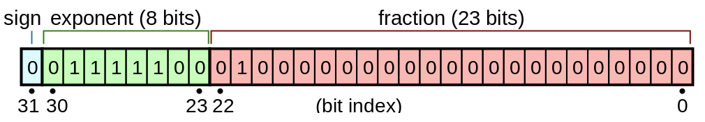
(Source)
Here are some links to further introductory material:
- A great explanation of how floats work: YouTube.
- This video works through adding two floats at the bit level: YouTube
Problems with Half-Precision
At high precision (FP32, FP64) you have enough breathing room that most of the time you don’t need to worry about the cases where the approximation falls apart and everything goes to hell. At FP16 you have to constantly think about the edge cases.
Let’s look at what FP16 looks like on a bit level:
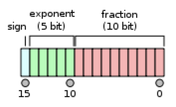
(Source)
- The exponent has 5 bits, giving it a range [-14, 15].
- Fraction has 10 bits.
- FP16 Range:
2^-14to2^15roughly - FP32 Range:
2^-126to2^127 - The ‘spaces’ between numbers is increased in FP16. There is a finite number of floats between 1 and 2, and
1 + 0.0001 = 1in FP16. This will cause problems during training. - When
update/param < 2^-11, updates will have no effect.
You can’t just use half-precision everywhere, because you will almost always get hit by one of the problems above. Instead we do what’s call mixed precision training. This is where you drop down to FP16 in some parts of the training and revert to FP32 to preserve precision in others.
We do the forward pass and the backwards pass in FP16, and pretty much everywhere else we use FP32. For example, when we apply the gradients in the weight update we use full precision. Accumulate in FP32 and store in FP16.
There are still some problems remaining if we do this:
- Weight update is imprecise.
1+0.0001 = 1=> vanishing gradients. - Gradients can underflow. Numbers get too low, get replaced by 0 => vanishing gradients.
- Activations, loss, or reductions can overflow => Makes NaNs, training diverges.
The following subsections show how these are addressed.
Master Copy of Weights
To solve the first problem listed above - weight update is imprecise - we can store a ‘master’ copy of the weights in FP32. It is this that gets passed to the optimizer:
opt = torch.optim.SGD(master_params, lr=1e-3)
After the optimizer step you then copy the master weights back into the model weights in FP16: master.grad.data.copy_(model.grad.data)
Then, our training loop will look like:
- Compute the output with the FP16 model, then the loss
- Back-propagate the gradients in half-precision.
- Copy the gradients in FP32 precision
- Do the update on the master model (in FP32 precision)
- Copy the master model in the FP16 model.
Loss Scaling
Next we need to tackle the second problem - gradients can underflow when doing backprop in FP16. To avoid the gradients getting zeroed by the FP16 precision, we multiply the loss by a scale factor. Typically this factor is something like 512 or 128.
We want to do this because the activation gradient values are typically very small and so fall outside of FP16’s representable range. Here is a histogram of the magnitude of activation gradients:
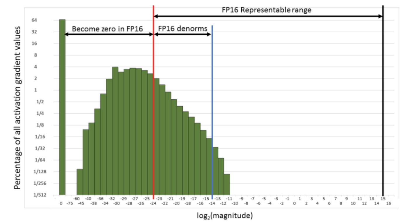
What we want to do is push that distribution to the right and into the representable range of FP16. We could do this by multiplying the loss by 512 or 1024.
We don’t want these 512-scaled gradients to be in the weight update, so after converting them to FP32, we need to ‘descale’ by dividing by the scale factor.
The training loop changes to:
- Compute the output with the FP16 model, then the loss.
- Multiply the loss by scale then back-propagate the gradients in half-precision.
- Copy the gradients in FP32 precision then divide them by scale.
- Do the update on the master model (in FP32 precision).
- Copy the master model in the FP16 model.
Accumulate to FP32
The last problem - Activations, loss, or reductions can overflow - needs to be dealt with in a couple of places.
First, the loss can overflow, so let’s do the reduction calculation that gives the loss in FP32:
y_pred = model(x) # y_pred: fp16
loss = F.mse_loss(y_pred.float(), y.float()) # loss is now FP32
scaled_loss = scale_factor * loss
Another overflow risk is occurs with Batchnorm, which also should do its reduction in FP32. You can recursively go through your model and change all the Batchnorm layers back to FP32 with this function:
bn_types = (nn.BatchNorm1d, nn.BatchNorm2d, nn.BatchNorm3d)

def bn_to_float(model):
    if isinstance(model, bn_types): model.float()
    for child in model.children():  bn_to_float(child)
    return model
You can then convert your Pytorch model to half precision with this function:
def model_to_half(model):
    model = model.half()
    return bn_to_float(model)
Dynamic Loss Scaling
The problem with loss scaling is that it has a magic number, the scale_factor, that you have to tune. As the model trains, different values may be necessary. Dynamic loss scaling is a technique that adaptively sets the scale_factor to the right value at runtime. This value will be perfectly fitted to our model and can continue to be dynamically adjusted as the training goes, if it’s still too high, by just halving it each time we overflow. After a while though, training will converge and gradients will start to get smaller, so we also need a mechanism to get this dynamic loss scale larger if it’s safe to do so.
Algorithm:
- First initialize
scale_factorwith a really high value, e.g. 512. - Do a forward and backward pass.
- Check if any of the gradients overflowed.
- If any gradients overflowed, half the
scale_factor, and zero the gradients (thus skipping the optimization step). - If the loop goes 500 steps without an overflow, double the
scale_factor.
How do we test for overflow? A useful property of NaNs is that they propagate - add anything to a NaN and the result if NaN. So if we sum a tensor that contains a Nan the result will be NaN. To check if it is NaN we can use the counter-intuitive property that NaN!=NaN and simply check if the result of the sum equals itself. Here is the code:
def test_overflow(x):
    s = float(x.float().sum())
    return (s == float('inf') or s == float('-inf') or s != s)
Summary
Here is a diagram of the mixed precision training loop containing all the above described steps:
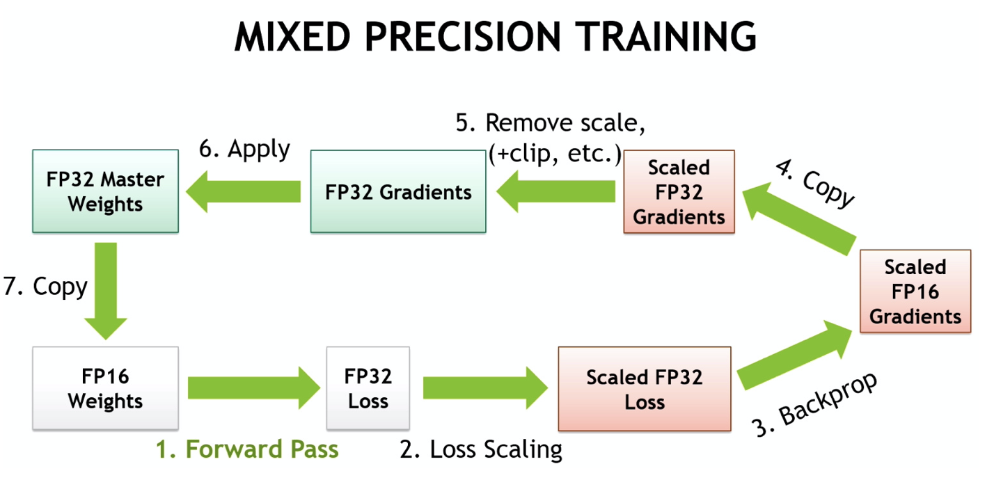
(Source: NVIDIA - Mixed-Precision Training Techniques Using Tensor Cores for Deep Learning)
In conclusion, here are the 3 problems caused by converting the model with FP16 and how they are mitigated:
Weight update is imprecise=> “Master” weights in FP32Gradients can underflow=> Loss (gradient) scalingActivations or loss can overflow=> Accumulate in FP32
Sometimes training with half-precision gives better results. More randomness, some regularization. Often the results are similar to what you get with FP32, but just faster.
Implementing Mixed Precision with APEX
APEX is a utility library authored by NVIDIA for doing mixed precision and distributed training in Pytorch.
APEX can convert a model to FP16, keeping the batchnorm’s at FP32, with the function:
import apex.fp16_utils as fp16

model = fp16.convert_network(model, torch.float16)
From the model parameters (mostly in FP16), APEX can create a master copy in FP32 that we will use for the optimizer step:
model_p, master_p = fp16.prep_param_lists(model)
After the backward pass, all gradients must be copied from the model to the master params before the optimizer step can be done in FP32:
fp16.model_grads_to_master_grads(model_p, master_p)
After the optimizer step we need to copy back the master parameters to the model parameters for the next update:
fp16.master_params_to_model_params(model_params, master_params)
If you want to use parameter groups then we need to do a bit more work than this. Parameter groups allow you to do things like:
- Transfer learning and freeze some layers
- Apply discriminative learning rates
- Don’t apply weight decay to some layers (like BatchNorm) or the bias terms
Parameter groups are the business of the optimizer not the model, so we need to define a new prep_param_lists that takes the optimizer and returns the model and master params grouped in a nested list. Then you need too define wrappers for model_grads_to_master_grads and master_params_to_model_params that work on these nested lists. It’s straight-forward, but I won’t reproduce it here. It is shown in the notebook: 10c_fp16.ipynb
Callback Implementation
Mixed precision training as a callback with dynamic loss scaling:
class MixedPrecision(Callback):
    _order = 99
    def __init__(self, loss_scale=512, flat_master=False, dynamic=True, max_loss_scale=2.**24, div_factor=2.,
                 scale_wait=500):
        assert torch.backends.cudnn.enabled, "Mixed precision training requires cudnn."
        self.flat_master,self.dynamic,self.max_loss_scale = flat_master,dynamic,max_loss_scale
        self.div_factor,self.scale_wait = div_factor,scale_wait
        self.loss_scale = max_loss_scale if dynamic else loss_scale

    def begin_fit(self):
        self.run.model = fp16.convert_network(self.model, dtype=torch.float16)
        self.model_pgs, self.master_pgs = get_master(self.opt, self.flat_master)
        #Changes the optimizer so that the optimization step is done in FP32.
        self.run.opt.param_groups = self.master_pgs #Put those param groups inside our runner.
        if self.dynamic: self.count = 0

    def begin_batch(self): self.run.xb = self.run.xb.half() #Put the inputs to half precision
    def after_pred(self):  self.run.pred = self.run.pred.float() #Compute the loss in FP32
    def after_loss(self):
        if self.in_train: self.run.loss *= self.loss_scale #Loss scaling to avoid gradient underflow

    def after_backward(self):
        #First, check for an overflow
        if self.dynamic and grad_overflow(self.model_pgs):
            #Divide the loss scale by div_factor, zero the grad (after_step will be skipped)
            self.loss_scale /= self.div_factor
            self.model.zero_grad()
            return True #skip step and zero_grad
        #Copy the gradients to master and unscale
        to_master_grads(self.model_pgs, self.master_pgs, self.flat_master)
        for master_params in self.master_pgs:
            for param in master_params:
                if param.grad is not None: param.grad.div_(self.loss_scale)
        #Check if it's been long enough without overflow
        if self.dynamic:
            self.count += 1
            if self.count == self.scale_wait:
                self.count = 0
                self.loss_scale *= self.div_factor

    def after_step(self):
        #Zero the gradients of the model since the optimizer is disconnected.
        self.model.zero_grad()
        #Update the params from master to model.
        to_model_params(self.model_pgs, self.master_pgs, self.flat_master)
XResNet
(Jump to Lesson 12 video); Notebook: 11_train_imagenette.ipynb
So far all of the image models we’ve used have been boring convolution models. What we really want to be using is a ResNet model. We will implement XResNet, which is the the mutant/extended version of ResNet. This is a tweaked ResNet taken from the Bag of tricks paper.
Let’s go through the XResNet modifications…
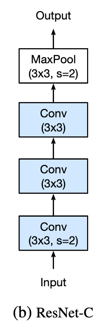
ResNet Stem Trick
ResNetC - don’t do a big 7x7 convolution at the start, because it’s inefficient and is just a single linear model. Instead do three 3x3 convs in a row. The receptive field is still going to be about 7x7, but it has a much richer number of things it can learn because it has 3 layers instead of 1. We call these first layers the stem. (This was also covered in Lesson 11)
-
The Conv layer takes in a number of input channels
c_inand outputs a number of output channelsc_out. - First layer by default has
c_in=3because normally we have RGB images. - We set the number of outputs to
c_out=(c_in+1)*8. This gives the second layer an input of 32 channels, which is what the bag of tricks paper recommends. - The factor of 8 also helps use the GPU architecture more efficiently. This grows / shrinks by itself with the number of input channels, so if you have more inputs then it will have more activations.
The first few layers are called the stem and it looks like:
nfs = [c_in, (c_out+1)*8, 64, 64] # c_in/c_outs for the 3 conv layers
stem = [conv_layer(nfs[i], nfs[i+1], stride=2 if i==0 else 1) for i in range(3)]
Where conv_layer is:
act_fn = nn.ReLU(inplace=True)


def conv(ni, nf, ks=3, stride=1, bias=False):
    return nn.Conv2d(ni, nf, kernel_size=ks, stride=stride, padding=ks//2, bias=bias)


def conv_layer(ni, nf, ks=3, stride=1, zero_bn=False, act=True):
    bn = nn.BatchNorm2d(nf)
    nn.init.constant_(bn.weight, 0. if zero_bn else 1.) # init batchnorm trick
    layers = [conv(ni, nf, ks, stride=stride), bn]
    if act: layers.append(act_fn)
    return nn.Sequential(*layers)
conv_layer is a nn.Sequential object of:
- a convolution
- followed by a BatchNorm
- and optionally an activation (default ReLU)
Zero BatchNorm Trick
After the stem the remainder of the ResNet’s body is an arbitrary number of ResBlocks. In the ResBlock there is one extra trick with the BatchNorm initialization. We sometimes initialize the BatchNorm weights to be 0 and other times we initialize it to 1.
To get why this would be useful, recall the diagram of the standard ResBlock:
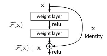
Each ‘weight layer’ in the above is a Conv/BatchNorm. If the input to a ResBlock is x then its output is x+block(x). If we initialize the final BatchNorm layer in the block to 0, then this is the same as multiplying the input by 0, so block(x)=0. Therefore at the start of training all ResBlocks just return their inputs, and this mimics a network that has fewer layers and is easier to train at the initial stage.
ResBlock
After the stem the remainder of the ResNet’s body is an arbitrary number of ResBlocks. The ResBlock code:
def noop(x): return x  # identity operation

class ResBlock(nn.Module):
    def __init__(self, expansion, ni, nh, stride=1):
        # expansion = 1 or 4
        super().__init__()
        nf,ni = nh*expansion,ni*expansion
        layers  = [conv_layer(ni, nh, 3, stride=stride),
                   conv_layer(nh, nf, 3, zero_bn=True, act=False)
        ] if expansion == 1 else [
                   conv_layer(ni, nh, 1),
                   conv_layer(nh, nh, 3, stride=stride),
                   conv_layer(nh, nf, 1, zero_bn=True, act=False)
        ]
        self.convs = nn.Sequential(*layers)
        self.idconv = noop if ni==nf else conv_layer(ni, nf, 1, act=False)
        self.pool = noop if stride==1 else nn.AvgPool2d(2, ceil_mode=True)

    def forward(self, x):
        return act_fn(self.convs(x) + self.idconv(self.pool(x)))
There several different types of ResBlocks in a ResNet and these are all contained in the comlete ResBlock code above, conditional on parameters expansion and stride.
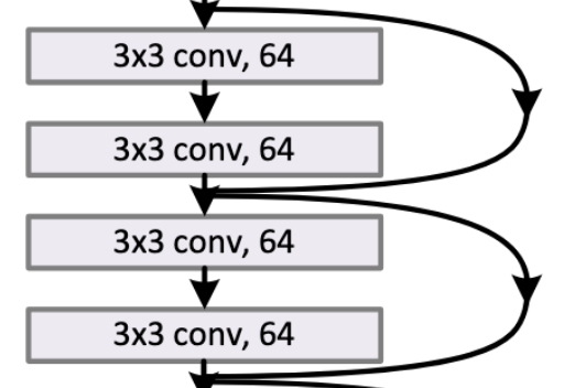
There is the standard ResBlock that has expansion=1 and stride=1 that are stacked together in ResNet18/30, like those in this diagram:
Besides the standard there are two other ResBlocks - the Expansion (AKA Bottleneck) ResBlock, and the Downsampling ResBlock. Let’s go through them and how they are tweaked by the Bag of Tricks paper.
Expansion/BottleNeck ResBlock
For ResNet18/34 the ResBlock looks like the diagram on the left below - a tensor comes in with shape [*, *, 64] and undergoes two 3x3 conv_layers. However, for the deeper ResNets (e.g. 50+) doing all these 3x3 conv_layers is expensive and costs memory. Instead we use a BottleNeck that has a 1x1 convolution to squish number of channels down by 4, then we do a single 3x3 convolution, followed by another 1x1 to project it back up to the original shape. Since we are squishing the number of channels down by a factor of 4 in the 3x3 conv_layer, we expand the normal number of channels in the model by a factor of 4 to get the equivalent size of the convolution as the basic block. See the diagram on the right below:
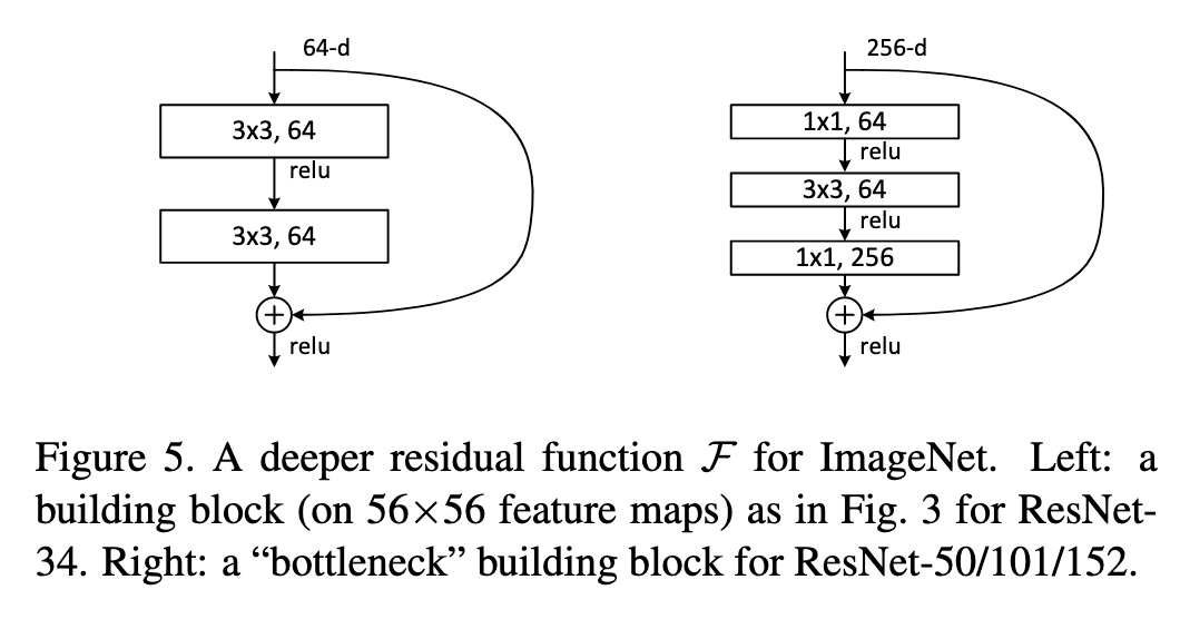
(Diagram taken from the original ResNet paper)
In the ResBlock code, this bottleneck layer is implemented through the expansion parameter. expansion is either 1 or 4. We multiple the number of input and output channels by this factor: nf,ni = nh*expansion,ni*expansion. This factor is 4 for ResNet50+.
Downsampling ResBlock
At the start of a new group of ResBlocks we typically half the spatial dimensions with a stride 2 convolution and also double the number of channels. The dimensions have now changed so what happens to the identity connection? In the original paper they use a projection matrix to reduce the dimensions, and other implementions I’ve seen use a 1x1 conv_layer with stride 2.
The way they do it in the bag of tricks paper is to do an AveragePooling layer with stride 2 to half the grid size, followed by a 1x1 conv_layer (stride 1) to increase the number of channels. Here is a diagram of the downsampling ResBlock:
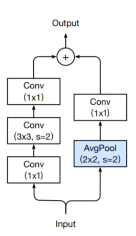
A further tweak, which is shown above, is putting the stride 2 in the 3x3 conv_layer. Prior to this, people the stride 2 in the first 1x1 conv_layer, which is a terrible thing to do because you are just throwing away 3 quarters of the data.
Putting it Together
Here is the code for creating any ResNet model:
class XResNet(nn.Sequential):
    @classmethod
    def create(cls, expansion, layers, c_in=3, c_out=1000):
        nfs = [c_in, (c_in+1)*8, 64, 64]
        stem = [conv_layer(nfs[i], nfs[i+1], stride=2 if i==0 else 1)
            for i in range(3)]

        nfs = [64//expansion,64,128,256,512]
        res_layers = [cls._make_layer(expansion, nfs[i], nfs[i+1],
                                      n_blocks=l, stride=1 if i==0 else 2)
                  for i,l in enumerate(layers)]
        res = cls(
            *stem,
            nn.MaxPool2d(kernel_size=3, stride=2, padding=1),
            *res_layers,
            nn.AdaptiveAvgPool2d(1), Flatten(),
            nn.Linear(nfs[-1]*expansion, c_out),
        )
        init_cnn(res)
        return res

    @staticmethod
    def _make_layer(expansion, ni, nf, n_blocks, stride):
        return nn.Sequential(
            *[ResBlock(expansion, ni if i==0 else nf, nf, stride if i==0 else 1)
              for i in range(n_blocks)])
Combined with the ResBlock code that is all that is required for creating any ResNet model. :)
Now we can create all of our ResNets by listing how many blocks we have in each layer and the expansion factor (4 for 50+):
def xresnet18 (**kwargs): return XResNet.create(1, [2, 2,  2, 2], **kwargs)
def xresnet34 (**kwargs): return XResNet.create(1, [3, 4,  6, 3], **kwargs)
def xresnet50 (**kwargs): return XResNet.create(4, [3, 4,  6, 3], **kwargs)
def xresnet101(**kwargs): return XResNet.create(4, [3, 4, 23, 3], **kwargs)
def xresnet152(**kwargs): return XResNet.create(4, [3, 8, 36, 3], **kwargs)
Image Classification: Transfer Learning / Fine Tuning
(Jump_to lesson 12 video), (Notebook: 11a_transfer_learning.ipynb)
Recall the familiar ‘one-two’ training combo from part 1 of fastai for getting good results on Image classification tasks:
- Get pretrained ResNet weights
- Create a new ‘head’ section of the model for your new task.
- Freeze all the layers except the head.
- Run a few cycles of training for the head.
- Unfreeze all the layers and run a few more training cycles.
Let’s implement the code required to make that possible.
Custom Head
In the notebook they want to use a model pretrained on ImageWoof to fine tune for the Pets dataset. We can save our ImageWoof model to disk as a dictionary of layer_name: tensor. PyTorch model has this readily available with st = learn.model.state_dict().
Let’s go through the process of loading back in the pretrained ImageWoof model. First we need to create a Learner:
learn = cnn_learner(xresnet18, data, loss_func, opt_func, c_out=10, norm=norm_imagenette)
ImageWoof has 10 activations, so we need to match this so the weights match up: c_out=10.
We can then load the ImageWoof state dictionary and load the weights into our Learner:
st = torch.load('imagewoof')
m = learn.model
m.load_state_dict(st)
This is now just the recovered ImageWoof model. We want to change it so it can be used on the new dataset, so we take off the last linear layer for 10 classes and replace it with one for the 37 classes of the Pets dataset. We can find the point we want to cut the model by searching for the index cut that points to the nn.AdaptiveAvfPool2d layer, which is the penultimate layer before the head. The cut model is then: m_cut = m[:cut].
The number of outputs of our new head is 37, what about the inputs? We can determine that easily by just running a batch through the cut model: ni = m_cut(xb).shape[1].
We can now create our new head for the Pets model:
m_new = nn.Sequential(
    m_cut, AdaptiveConcatPool2d(), Flatten(),
    nn.Linear(ni*2, 37))
Where we also use AdaptiveConcatPool2d which is simply average pooling and max pooling catted together into a 2*ni sized vector. This double pooling is a fastai trick that gives a little boost over just doing one of the other.
class AdaptiveConcatPool2d(nn.Module):
    def __init__(self, sz=1):
        super().__init__()
        self.output_size = sz
        self.ap = nn.AdaptiveAvgPool2d(sz)
        self.mp = nn.AdaptiveMaxPool2d(sz)
    def forward(self, x): return torch.cat([self.mp(x), self.ap(x)], 1)
With this simple transfer learning we can get 71% on Pets after 4 epochs. Without the transfer learning we only get 37%.
All the steps together: put this whole process in a function:
def adapt_model(learn, data):
    cut = next(i for i,o in enumerate(learn.model.children())
               if isinstance(o,nn.AdaptiveAvgPool2d))
    m_cut = learn.model[:cut]
    xb,yb = get_batch(data.valid_dl, learn)
    pred = m_cut(xb)
    ni = pred.shape[1]
    m_new = nn.Sequential(
        m_cut, AdaptiveConcatPool2d(), Flatten(),
        nn.Linear(ni*2, data.c_out))
    learn.model = m_new
Then the weight loading and model adaption is simply becomes:
learn = cnn_learner(xresnet18, data, loss_func, opt_func, c_out=10, norm=norm_imagenette)
learn.model.load_state_dict(torch.load(mdl_path/'iw5'))
adapt_model(learn, data)
Freezing Layers
You can freeze layers by turning their gradients off:
for p in learn.model[0].parameters(): p.requires_grad_(False)
Let’s do one-two training combo.
- Freezing the body and training the head 3 epochs gets 54%.
- Unfreezing and training the rest of the model for another 5 epochs gets 56%(!)
It’s better than not fine tuning, but interestingly when we just fine-tuned without the freezing we got a way better result of 71%. Why doesn’t it work?
Every time something weird happens in your neural net, it’s almost certainly due to batchnorm. Because batchnorm makes everything weird. :D
The batchnorm layers in the pretrained model have learned means and stds for a different dataset (ImageWoof). When we trained froze the body and trained the head, the head was learning with a different set of batch norm statistics. When we unfreeze the body the batchnorm statistics can now change, which effectively causes the ground to shift from underneath the later layers that we just changed.
Fix: Don’t freeze the weights in the batchnorm layers when doing partial layer training.
Here’s the function that does the freezing and unfreezing of layers, which skips batchnorm layers:
def set_grad(m, b):
    if isinstance(m, (nn.Linear,nn.BatchNorm2d)): return
    if hasattr(m, 'weight'):
        for p in m.parameters(): p.requires_grad_(b)
We can use PyTorch apply method to apply this function to our model:
learn.model.apply(partial(set_grad, b=False));
ULMFiT From Scratch
ULMFiT is transfer learning applied to AWD-LSTM for NLP
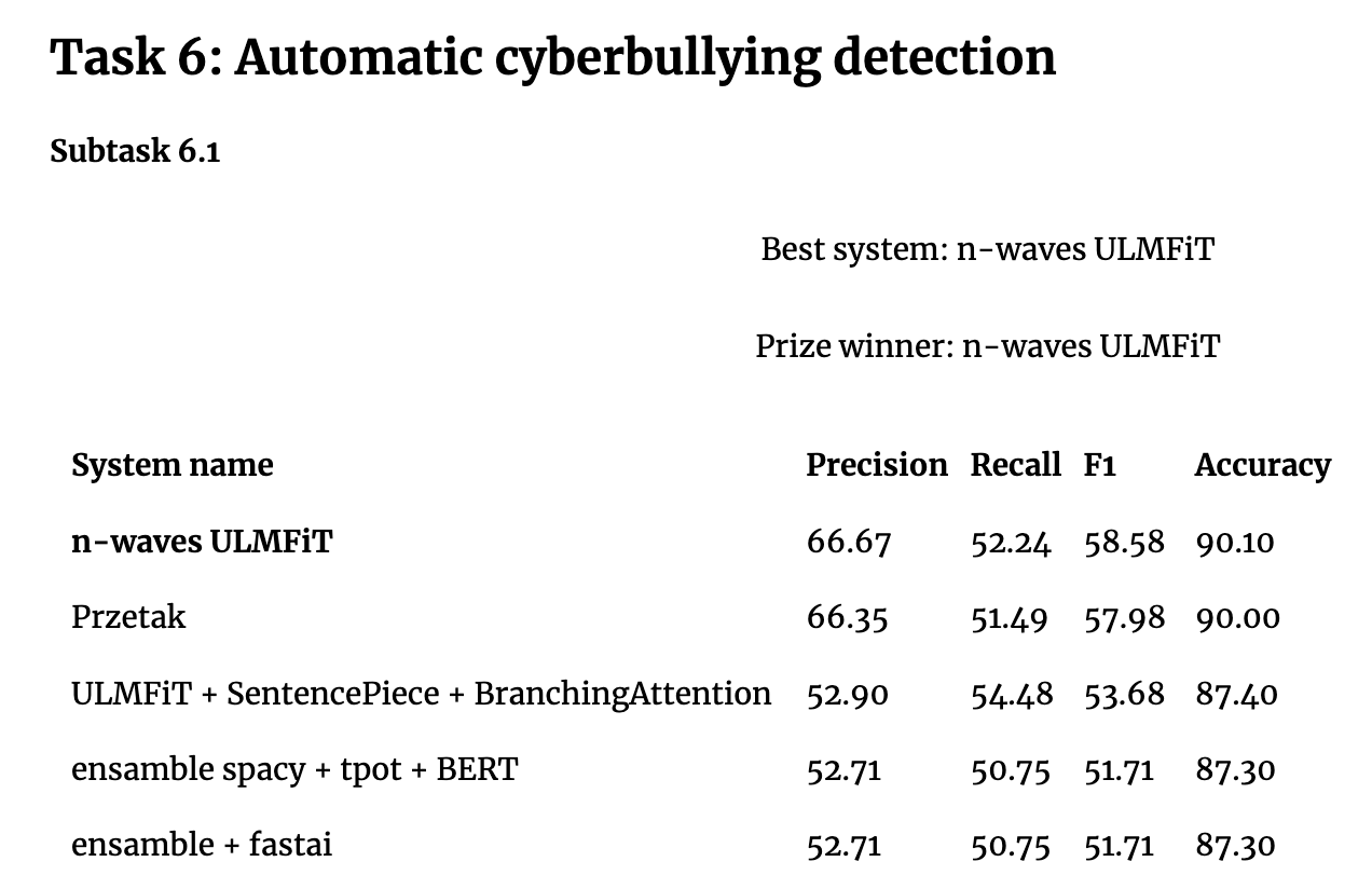
There has been a lot of ground-breaking innovation in the realm of transfer learning applied to NLP recently - e.g. GPT2, BERT. These are all based on Transformers, which are currently very hot, so one could think that LSTMs aren’t used or interesting anymore. However when you look at recent competitive machine learning results (NB recorded 2019), you see ULMFiT beating BERT - from poleval2019:
Jeremy says…:
It’s definitely not true that RNNs are in the past. Transformers and CNNs for text have a lot of problems. They don’t have state. So if you are doing speech recognition, for every sample you look at you have to do an entire analysis of all the sample around it again and again and again. So it’s rediculously wasteful. Wheras RNNs have state. But they are fiddly and hard to deal with when you want to do research and change things. RNNs, and in particular AWD-LSTM, have had a lot of research done on how to regularize them carefully. Stephen Merity did a huge amount of work on all the different way they can be regularized. There is nothing like that outside the RNN world. At the moment my goto choice is still ULMFiT for most real world tasks. I’m not seeing transformers win competitions yet.
There are lots of things that are sequences that aren’t text - genomics, chemical bonding analysis, and drug discovery. People are finding exciting applications of ULMFiT outside of NLP.
Here is a review of the ULMFiT pipeline that we saw in part 1 of fastai v3:
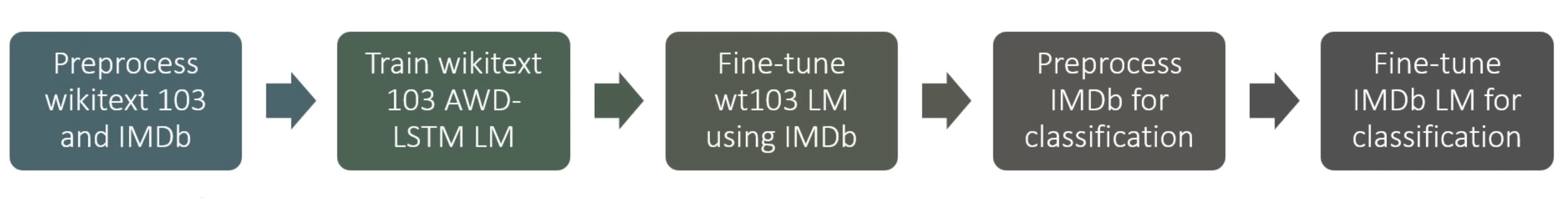
We are going to code this up from scratch…
Preprocess Text
Notebook: 12_text.ipynb
We will use the IMDB dataset that consists of 50,000 labeled reviews of movies (positive or negative) and 50,000 unlabelled ones. It contains a train folder, a test folder, and an unsup (unsupervised) folder.
First thing we need to do is create a datablocks ItemList subclass for text:
def read_file(fn):
    with open(fn, 'r', encoding = 'utf8') as f: return f.read()

class TextList(ItemList):
    @classmethod
    def from_files(cls, path, extensions='.txt', recurse=True, include=None, **kwargs):
        return cls(get_files(path, extensions, recurse=recurse, include=include), path, **kwargs)

    def get(self, i):
        if isinstance(i, Path): return read_file(i)
        return i
This was easy because we reuse much code we wrote previously. We already have the get_files function, which now searches for .txt files instead of images. Then we override get to now call a function, read_file that reads a text file. Now we can load the dataset:
il = TextList.from_files(path, include=['train', 'test', 'unsup'])
If we look at one of the items it will be just the raw text of a IMDB movie review.
We can just throw this in to a model - it needs to be numbers. So we need to Tokenize and Numericalize it.
Tokenizing
We need to tokenize the dataset first, which is splitting a sentence in individual tokens. Those tokens are the basic words or punctuation signs with a few tweaks: don't for instance is split between do and n't. We will use a processor for this, in conjunction with the spacy library.
Before tokenizing, we will apply a bit of preprocessing on the texts to clean them up (we saw the one up there had some HTML code). These rules are applied before we split the sentences in tokens.
default_pre_rules = [fixup_text, replace_rep, replace_wrep,
                     spec_add_spaces, rm_useless_spaces, sub_br]

default_spec_tok = [UNK, PAD, BOS, EOS, TK_REP,
                    TK_WREP, TK_UP, TK_MAJ]
These are:
fixup_text: Fixes various messy things seen in documents. For example, HTML artifacts.replace_rep: Replace repetitions at the character level:!!!!!->TK_REP 5 !replace_wrep: Replace word repetitions:word word word->TK_WREP 3 wordspec_add_spaces: Add spaces around/and#rm_userless_spaces: If we find more than two spaces in a row, replace them with one spacesub_br: Replaces the<br />by\n
Why do replace_rep and replace_wrep? Let’s image a tweet that said: “THIS WAS AMAZING!!!!!!!!!!!!!!!!!!!!!”. We could treat the exclamation marks as one token, so we would then have a single vocab item that is specifically 21 exclamation marks. You probably wouldn’t see that again so it wouldn’t even end up in your vocab, and if it did it would be so rare that you wouldn’t be able to learn anything interesting about it. It would also absurdly be different from the case where there is 20 or 22 exclamation marks. But some big number of exclamation marks does have a meaning and we know that it is different from the case where there is just a single one. If we instead replace it with ` xxrep 21 ! `, then this is just three tokens where the model can learn that lots of repeating exclamation marks is a general concept that has certain semantics to it.
Another alternative would be to turn our sequence of exclamation marks into 21 tokens in a row, but now we are asking our LSTM to hang onto that state for 21 timesteps, which is a lot more work for it to do and it won’t do as good a job.
What we are trying to do in NLP is to make it so that the things in our vocabulary are as meaningful as possible.
After tokenizing with spacey we apply a couple more rules:
replace_all_caps: Replace tokens in ALL CAPS by their lower version and insertTK_UPbefore.deal_caps: Replace all Captitalized tokens by their lower version and addTK_MAJbefore.add_eos_bos: Add before-stream (BOS) and end-of-stream (EOS) tokens on either side of a list of tokens at the start/end of a document. These tokens turn out to be very important. When the model encounters aEOStoken it knows it is at the end of a document and that the next document is something new. So it will have to learn to reset its state somehow.
For example:
> replace_all_caps(['I', 'AM', 'SHOUTING'])
['I', 'xxup', 'am', 'xxup', 'shouting']


> deal_caps(['My', 'name', 'is', 'Jeremy'])
['xxmaj', 'my', 'name', 'is', 'xxmaj', 'jeremy']
Tokenizing with spacey is quite slow because spacey does things very carefully. spacey has a sophisticated parser based tokenizer and it using it will improve your accuracy a lot, so it’s worth using. Luckily tokenizing is embarrassingly parallel so we can speed things up using multi-processing.
class TokenizeProcessor(Processor):
    def __init__(self, lang="en", chunksize=2000, pre_rules=None, post_rules=None, max_workers=4):
        self.chunksize,self.max_workers = chunksize,max_workers
        self.tokenizer = spacy.blank(lang).tokenizer
        for w in default_spec_tok:
            self.tokenizer.add_special_case(w, [{ORTH: w}])
        self.pre_rules  = default_pre_rules  if pre_rules  is None else pre_rules
        self.post_rules = default_post_rules if post_rules is None else post_rules

    def proc_chunk(self, args):
        i,chunk = args
        chunk = [compose(t, self.pre_rules) for t in chunk]
        docs = [[d.text for d in doc] for doc in self.tokenizer.pipe(chunk)]
        docs = [compose(t, self.post_rules) for t in docs]
        return docs

    def __call__(self, items):
        toks = []
        if isinstance(items[0], Path): items = [read_file(i) for i in items]
        chunks = [items[i: i+self.chunksize] for i in (range(0, len(items), self.chunksize))]
        toks = parallel(self.proc_chunk, chunks, max_workers=self.max_workers)
        return sum(toks, [])

    def proc1(self, item):
        return self.proc_chunk([item])[0]

    def deprocess(self, toks):
        return [self.deproc1(tok) for tok in toks]

    def deproc1(self, tok):
        return " ".join(tok)
Here is what an example raw input looks like:
'Comedian Adam Sandler\'s last theatrical release "I Now Pronounce You Chuck and Larry" served as a loud and proud plea for tolerance of the gay community. The former "Saturday Night Live" funnyman\'s new movie "You Don\'t Mess with the Zohan" (*** out o'
And here’s what that looks like after tokenization:
'xxbos • xxmaj • comedian • xxmaj • adam • xxmaj • sandler • \'s • last • theatrical • release • " • i • xxmaj • now • xxmaj • pronounce • xxmaj • you • xxmaj • chuck • and • xxmaj • larry • " • served • as • a • loud • and • proud • plea • for • tolerance • of • the • gay • community • . • xxmaj • the • former • " • xxmaj • saturday • xxmaj • night • xxmaj • live • " • funnyman • \'s • new • movie •'
Numericalize Tokens
Once we have tokenized our texts, we replace each token by an individual number, this is called numericalizing. Again, we do this with a processor (not so different from the CategoryProcessor).
from collections import Counter


class NumericalizeProcessor(Processor):
    def __init__(self, vocab=None, max_vocab=60000, min_freq=2):
        self.vocab,self.max_vocab,self.min_freq = vocab,max_vocab,min_freq

    def __call__(self, items):
        #The vocab is defined on the first use.
        if self.vocab is None:
            freq = Counter(p for o in items for p in o)
            self.vocab = [o for o,c in freq.most_common(self.max_vocab) if c >= self.min_freq]
            for o in reversed(default_spec_tok):
                if o in self.vocab: self.vocab.remove(o)
                self.vocab.insert(0, o)

        if getattr(self, 'otoi', None) is None:
            self.otoi = collections.defaultdict(int,{v:k for k,v in enumerate(self.vocab)})
        return [self.proc1(o) for o in items]

    def proc1(self, item):
        return [self.otoi[o] for o in item]

    def deprocess(self, idxs):
        assert self.vocab is not None
        return [self.deproc1(idx) for idx in idxs]

    def deproc1(self, idx):
        return [self.vocab[i] for i in idx]
Tokenizing and Numericalizing text takes a while and so it’s best to do it once and then serialize it.
Batching Text for RNN Training
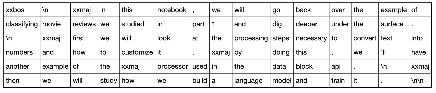
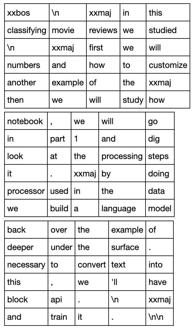
Batching up language model data requires a bit more care than it does with say image data. Let’s take work through batching with an example piece of text:
stream = """
In this notebook, we will go back over the example of classifying movie reviews we studied in part 1 and dig deeper under the surface.
First we will look at the processing steps necessary to convert text into numbers and how to customize it. By doing this, we'll have another example of the Processor used in the data block API.
Then we will study how we build a language model and train it.\n
"""
Let’s use a batch-size of 6. This sequences happens to divide into 6 pieces of length 15, so the length of our 6 sequences is 15.
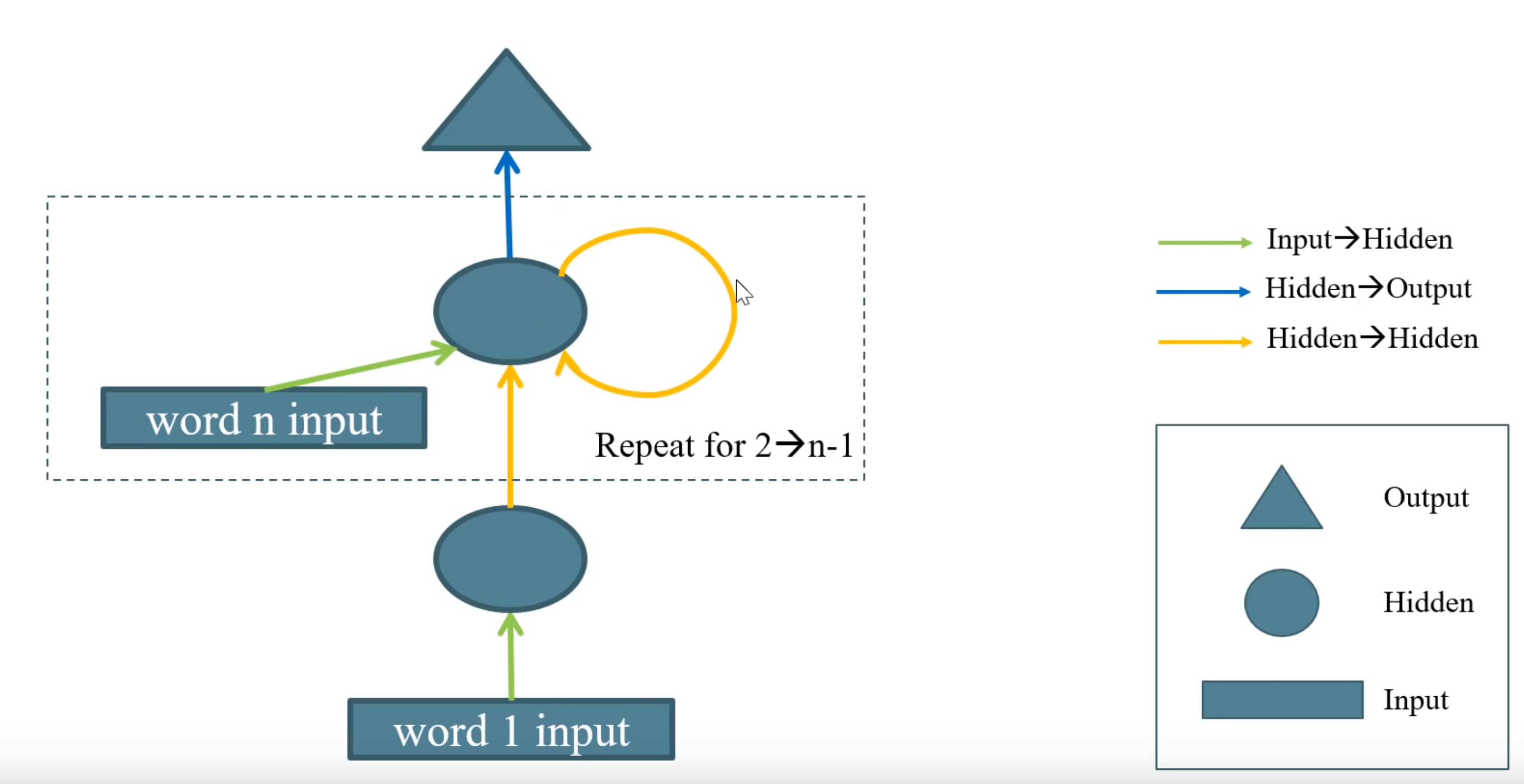
Every forward pass we will give our model chunks of text 5 tokens long. This is called the backpropagation through time (BPTT). This is a fancy sounding name, but it just means that every batch we view the RNN as being unfolded 5 times through time as shown below (source):

So the model would make 5 predictions for each mini-batch, accumulate the errors across the 5 time steps, then update the weights. (In other places this is called Truncated BPTT)
With bptt=5 we go over all the sequences in 3 mini-batches:
To reconstruct the order of the original text read the top row of all the batches, then the second, and so on.
The batch-size is like the number of texts that you train the model on in parallel. Along the rows of the batches, the text is in sequential order. This is essential because the model is creating an internal state that depends on what it is seeing. It needs to be in order.
What’s the difference between sequence length, batch-size, and bptt??
- Here is a brilliant graphic from Stefano Giomo that illustrates what these all mean.
Lets create a dataloader for language models. At the beginning of each epoch, it’ll shuffle the articles (if shuffle=True) and create a big stream by concatenating all of them. We divide this big stream in bs smaller streams. That we will read in chunks of bptt length.
What about the source x and target y of the language model task? For training our language model using self-supervised learning we want to take in a word and then predict the next word in the sequence. Therefore, the target y will be exactly the same as x, but shifted over by one word.
Let’s create this dataloader:
class LM_Dataset():
    def __init__(self, data, bs=64, bptt=70, shuffle=False):
        self.data,self.bs,self.bptt,self.shuffle = data,bs,bptt,shuffle
        total_len = sum([len(t) for t in data.x])
        self.n_batch = total_len // bs
        self.batchify()

    def __len__(self): return ((self.n_batch-1) // self.bptt) * self.bs

    def __getitem__(self, idx):
        source = self.batched_data[idx % self.bs]
        seq_idx = (idx // self.bs) * self.bptt
        # x, y (x shifted by 1 word)
        return source[seq_idx:seq_idx+self.bptt],source[seq_idx+1:seq_idx+self.bptt+1]

    def batchify(self):
        texts = self.data.x
        if self.shuffle: texts = texts[torch.randperm(len(texts))]
        stream = torch.cat([tensor(t) for t in texts])
        self.batched_data = stream[:self.n_batch * self.bs].view(self.bs, self.n_batch)
If we look at this, if x is:
"xxbos well worth watching , "
Then y would be:
"well worth watching , especially"
Question: What are the trade-offs to consider between batch-size and BPTT? For example, BTPP=10 vs BS=100, or BTPP=100 vs BS=10? Both would be passing 1000 tokens at a time to the model. What should you consider when tuning the ratio?
I don’t know the answer. This would make a super great experiment.
The batch-size is the the thing that lets it parallelize. So if your batch-size is small it’s just going to be super slow. On the other hand, a large batch size with a short bptt you may end up with less state that’s being backpropagated.
What the ratio should be - I’m not sure.
Batching Text for Training Classifiers
When we will want to tackle classification, gathering the data will be a bit different: first we will label our texts with the folder they come from. We’ve already done this for image models, and so we can reuse the code we already wrote for that:
proc_cat = CategoryProcessor()

il = TextList.from_files(path, include=['train', 'test'])
sd = SplitData.split_by_func(il, partial(grandparent_splitter, valid_name='test'))
ll = label_by_func(sd, parent_labeler, proc_x = [proc_tok, proc_num], proc_y=proc_cat)
The target/dependent variable could be the sentiment of the document: e.g. pos or neg.
Are we finished? Not quite.
When we worked with images, by the time we got to modelling they were all the same size (we resized them to a square). For texts, you can’t ignore that some texts are bigger than others. In order to collate a bunch of texts into a batch we will need to apply padding using some padding token to our documents so that documents collated into the same batches have the same length.
However, if we have a mini-batch with a 1000 word document, a 2000 word document, and then a 20 word document. The 20 word document is going to end up with 1980 padding tokens tacked onto the end. As we go through the RNN we are going to be calculating pointlessly on these padding tokens, which is a waste. So the trick is to sort the data first by length. That way your first mini-batch will contain your really long documents and your last mini-batch will contain your really short documents. This will mean that there won’t be much padding and wasted computation in any of the mini-batches.
In fastai this is done by creating a new type of Sampler. Naively, we can create a sampler that just sorts all our documents by length, but this would through away any randomness in constructing our batches - no shuffle. We can instead organize all the documents into buckets such that documents of similar size go in the same bucket. We can then do shuffling inside of those buckets to construct our mini-batches. This sampler is called SortishSampler in the lesson notebook.
Now we have shuffled the documents using SortishSampler we need to collate them into batches - i.e. stick them together into a batch tensor with a fixed known size. We add the padding token (that as an id of 1) at the end of each sequence to make them all the same size when batching them. Note that we need padding at the end to be able to use PyTorch convenience functions that will let us ignore that padding.
def pad_collate(samples, pad_idx=1, pad_first=False):
    max_len = max([len(s[0]) for s in samples])
    res = torch.zeros(len(samples), max_len).long() + pad_idx
    for i,s in enumerate(samples):
        if pad_first: res[i, -len(s[0]):] = LongTensor(s[0])
        else:         res[i, :len(s[0]) ] = LongTensor(s[0])
    return res, tensor([s[1] for s in samples])
So to create the data loader:
bs = 64
train_sampler = SortishSampler(ll.train.x, key=lambda t: len(ll.train[int(t)][0]), bs=bs)
train_dl = DataLoader(ll.train, batch_size=bs, sampler=train_sampler, collate_fn=pad_collate)
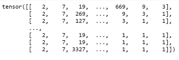
An example mini-batch looks like:
LSTM From Scratch
Now we will create an RNN. An RNN is like a network with many many layers. For, say, a document with 2000 words, it would be a network with 2000 layers. Of course, it is never explicitly code it that way and instead just use a for-loop.
Between every pair of hidden layers we use the same weight matrix. Problem is, trying to handle 2000 network layers we get vanishing gradients and exploding gradients and it’s really hard to get it to work. We can design more complex networks where the output of one RNN is fed into another RNN (stacked RNNs).
To get this thing to work, we need our hidden layers to do something more than just a matrix multiply. We instead use a LSTM Cell:
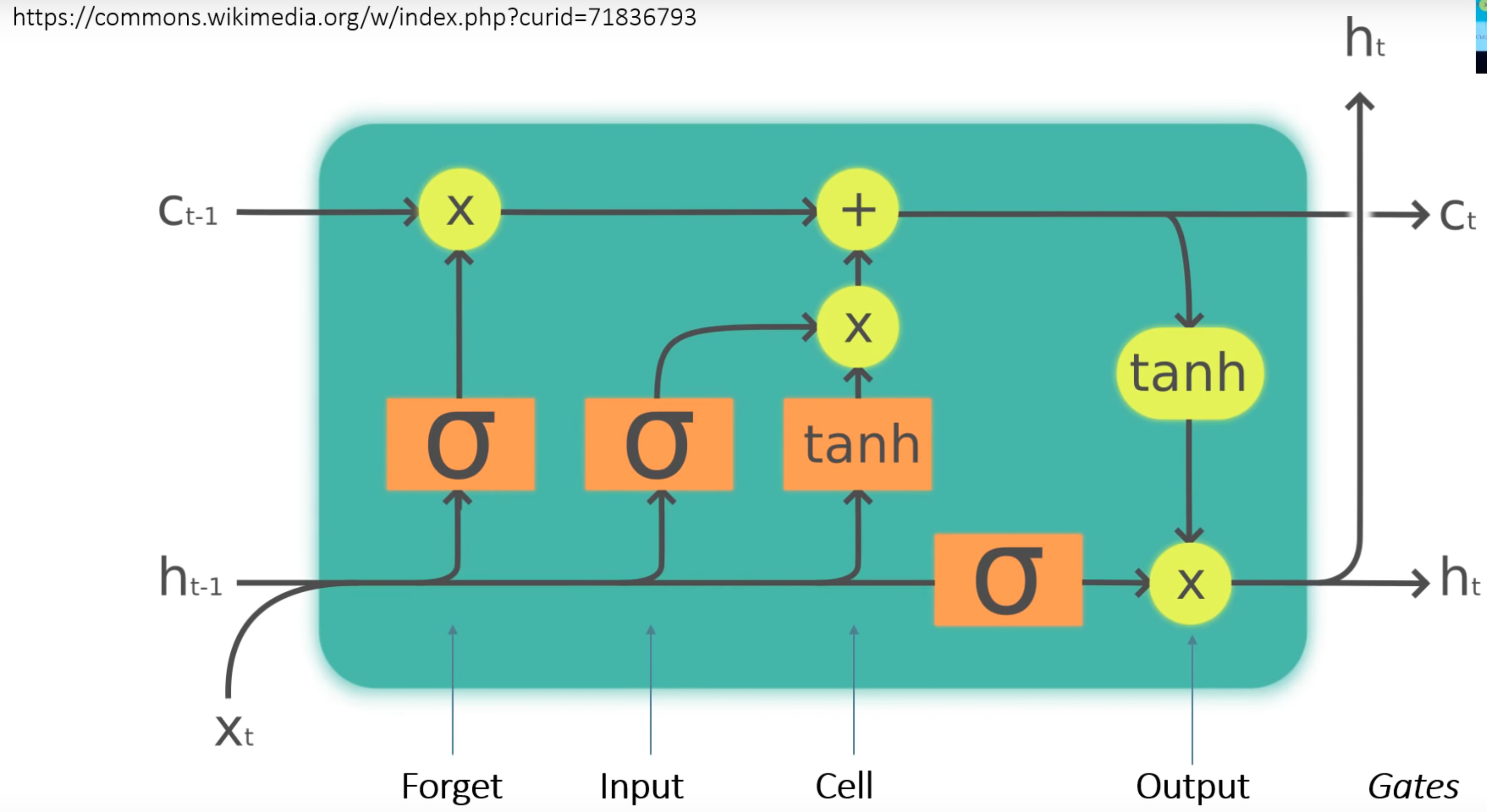
Recall that:
- Sigmoid function $\sigma$ - is a smooth function that goes from 0 to 1.
- Tanh function $\tanh$ - is a smooth function that goes from -1 to 1.
How to read this thing?
-
Starting from the bottom you have the input
xand the hidden layer output from the previous layerhcoming into the cell. -
xandhare fed into the orangesigmoidandtanhlayers simultaneously. The same values go into those layers. -
Each of those layers is basically another little hidden layer.
xandhare multiplied by matrices before going through thesigmoidortanhactivations. Each of the layers has its own matrices.
This diagram also includes equations that make it more clear:
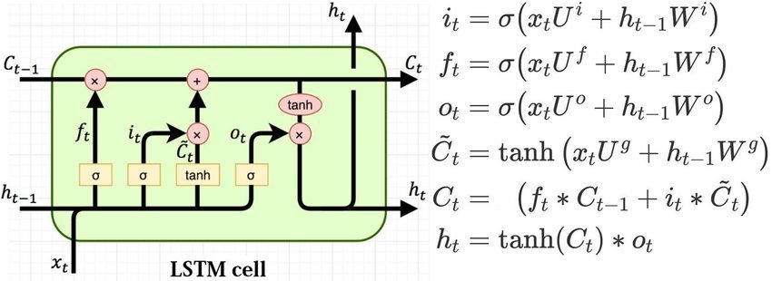
(picture from Understanding LSTMs by Chris Olah, definitely read this.)
Let’s follow the path through the cell:
- The forget path goes through a sigmoid and then hits the cell value, $C_{t-1}$. This is just a rank 2 tensor (with mini-batch) and represents the state or memory component of the LSTM that is passed on and updated through the timesteps.
- We multiply this by the output of the forget
sigmoid. So this gate has the ability to zero-out bits of the Cell state. We can look at some of our words coming in and say - based on that we should zero-out some of the Cell state. - We then add the selectively forgotten Cell state to the second little neural net. Here we have the outputs of two layers - a
sigmoidand a tanh - which are multiplied together and their product is then added to the selectively forgotten Cell state. - This part is where the LSTM chooses how to update the Cell state. This is carried through to the next time step as $C_t$.
- $C_t$ is then also put through another
tanhfunction and multiplied by our fourth and final mini neural net (anothersigmoid) to create the new output state $h_t$, that is passed on to the next time step. Thissigmoiddecides which parts of the Cell state to output.
It seems pretty weird, but as code it’s very simple to implement. In coding it, rather than have 4 different matrices for each of the internal mini neural nets, it’s more efficient to just stack them all into one 4x matrix and do one matmul. You can then split the output into equal sized chunks using the chunk function in PyTorch.
Here is the code for a LSTM cell:
class LSTMCell(nn.Module):
    def __init__(self, ni, nh):
        super().__init__()
        self.ih = nn.Linear(ni,4*nh) # input2hidden
        self.hh = nn.Linear(nh,4*nh) # hidden2hidden

    def forward(self, input, state):
        h,c = state
        #One big multiplication for all the gates is better than 4 smaller ones
        gates = (self.ih(input) + self.hh(h)).chunk(4, 1)
        ingate,forgetgate,outgate = map(torch.sigmoid, gates[:3])
        cellgate = gates[3].tanh()

        c = (forgetgate*c) + (ingate*cellgate)
        h = outgate * c.tanh()
        return h, (h,c)
Then an LSTM layer just applies the cell on all the time steps in order.
class LSTMLayer(nn.Module):
    def __init__(self, cell, *cell_args):
        super().__init__()
        self.cell = cell(*cell_args)

    def forward(self, input, state):
        inputs = input.unbind(1)
        outputs = []
        for i in range(len(inputs)):
            out, state = self.cell(inputs[i], state)
            outputs += [out]
        return torch.stack(outputs, dim=1), state
In practice this is:
lstm = LSTMLayer(LSTMCell, 300, 300)
x = torch.randn(64, 70, 300)
h = (torch.zeros(64, 300),torch.zeros(64, 300))
The hidden state and cell states are initialized with zeros at the start of training.
Aside: there are lots of other ways you can setup a layer that has the ability to selectively update and selectively forget things. For example, there is a popular alternative called a GRU, which has one less gate. The thing seems to be giving it some way to make the decision to forget things. Then it has the ability to not push state through all the thousands of time steps.
PyTorch’s LSTM Layer
We can now use the Pytorch’s own LSTM layer:
input_size, hidden_size, num_layers = 300, 300, 1
lstm = nn.LSTM(input_size,
               hidden_size,
               num_layers,
               batch_first=True)

bs, bptt = 64, 70
x = torch.randn(bs, bptt, input_size)
h = (torch.zeros(num_layers, bs, hidden_size),
     torch.zeros(num_layers, bs, hidden_size))

output, (h1, c1) = lstm(x, h)
It’s worth going over the dimensions because they confused me a lot.
Firstly, remember that this PyTorch module is not an individual LSTM cell, rather it is potentially multiple LSTM layers over multple timesteps. With PyTorch’s LSTM you can specify the num_layers and we also run it with bptt timesteps. The following diagram from this SO post shows how you should picture this:
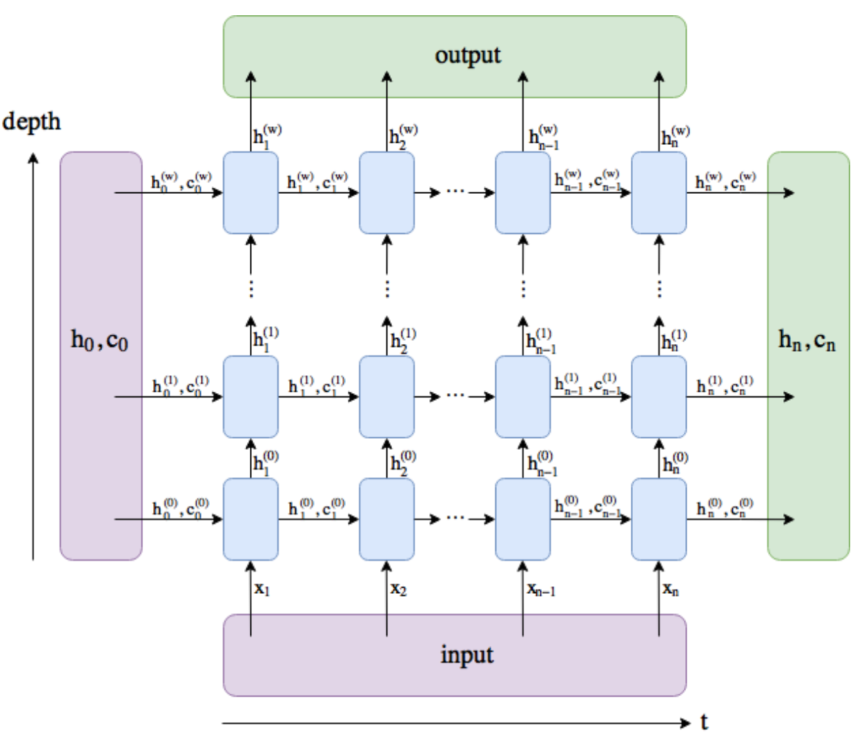
The depth is the num_layers and time is bptt.
The dimensions of the inputs:
input:(batch, bptt, input_size)h_0:(batch, num_layers, hidden_size)c_0:(batch, num_layers, hidden_size)
The dimensions of the outputs:
output:(batch, seq_len, hidden_size)h_n:(batch, num_layers, hidden_size)c_n:(batch, num_layers, hidden_size)
(NB this is while using batch_first=True)
AWD-LSTM
We want to use the AWD-LSTM from Stephen Merity et al. [2017]. In this paper, the authors thought about all the ways we can regularize and optimize the LSTM model for NLP. In their paper they test all the different kinds of way they can apply dropout to the LSTM.
- AWD-LSTM stands for: (Average Stochastic Gradient Descent)(Weight-Dropped)-LSTM…
Dropout consists of replacing some coefficients by 0 with probablility p. To ensure that the average of the weights remains constant, we apply a correction factor to the weights that aren’t nullified with value 1/(1-p).
def dropout_mask(x, sz, p):
    return x.new(*sz).bernoulli_(1-p).div_(1-p)
This looks like:
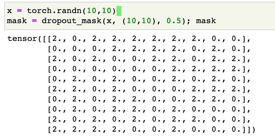
Once with have a dropout mask mask, applying the dropout to x is simply done by x = x * mask.
With RNN NLP tasks, a tensor x will have three dimensions:
- The
batch_size: the number of texts we are training on in parallel. - The
bptt: the number of tokens we are looking at at a time. - The
emb_size: the size of the vector representation of a token.
With (2, 3, 5) this could look like:
>> x = torch.randn(2,3,5)

tensor([[[ 0.1620,  0.0125, -0.5448, -0.8244,  0.3781],
         [ 0.2661, -0.7103, -0.5006,  0.5024,  0.7515],
         [-0.6798,  0.1970,  0.0260,  0.5037,  0.2735]],

        [[-0.0661,  1.2567, -1.2873, -1.1245,  0.0959],
         [-0.5627, -0.0315,  0.9382,  0.8043, -1.2791],
         [ 0.2626,  1.8968,  0.5332,  0.6908, -0.3327]]])
RNNDropout / Variational Dropout
For each document in the batch we want to have a unique dropout mask, but we also don’t want to randomly apply it on the vocab dimension, so that every token has a different dropout mask. We have a sequence length of say 5, then recall that the RNN will only do a single forward/backward/update pass with those 5.
Therefore the model needs to be the same for all those sequences and so we need to apply the same dropout mask on the entire sequence, otherwise it’s just broken.
The standard dropout can’t do this for us so we need to create our own layer called RNNDropout. We want to have different dropout masks for each member of the batch (document), but replicate it over their sequences. We can elegantly do this with a clever broadcasting trick, where you specify that the dropout mask has shape (x.size(0), 1, x.size(2)). That way when you multiply by the mask, it will be replicated down the sequence dimension.
class RNNDropout(nn.Module):
    def __init__(self, p=0.5):
        super().__init__()
        self.p=p

    def forward(self, x):
        if not self.training or self.p == 0.: return x
        m = dropout_mask(x.data, (x.size(0), 1, x.size(2)), self.p)
        return x * m
The output looks like:
>> x = torch.randn(5,3,5)
>> dp = RNNDropout(0.2)
>> dp(x)

tensor([[[-1.6986, -0.2667,  0.5033, -0.0000, -0.7446],
         [-1.5847, -0.1816,  2.8067, -0.0000,  0.1114],
         [ 0.4601,  0.6553,  1.4082,  0.0000, -1.6506]],

        [[ 1.7197, -1.0774,  0.0000,  0.1192, -0.0000],
         [ 0.9075, -0.1597,  0.0000, -1.3051,  0.0000],
         [ 0.5267,  1.0956,  0.0000, -2.3911, -0.0000]],

        [[ 0.0000, -0.0000,  0.6468,  1.8105,  0.6677],
         [ 0.0000,  0.0000, -0.6478,  0.8841, -2.5549],
         [ 0.0000,  0.0000,  1.1027,  0.7640, -0.4295]],

        [[-2.8382,  0.0000,  0.6135,  0.1007,  0.0000],
         [-0.7681,  0.0000, -1.1549, -1.4484, -0.0000],
         [ 1.5333,  0.0000,  1.0678, -1.4169, -0.0000]],

        [[ 0.0000, -0.2658, -0.0000,  0.0000,  0.3604],
         [-0.0000, -1.2424, -0.0000, -0.0000,  3.5358],
         [ 0.0000,  0.7004, -0.0000, -0.0000, -0.5376]]])
Note the positions of the 0s.
Weight Dropout / DropConnect
Weight dropout applies dropout not on the activations, but on the weights themselves. But otherwise the aim of regularization is the same as normal dropout. This is also called DropConnect. Here this is applied to the weights of the inner LSTM hidden to hidden matrix - $U^i, U^f, U^o, U^g$.
The DropConnect paper says:
DropConnect is the generalization of Dropout in which each connection, instead of each output unit as in Dropout, can be dropped with probability
p.
Since there are many more weights than activations to disable, DropConnect creates many more ways of altering the model.(Also see this Stackoverflow question on the difference between the two.)
The downside is that it requires us to keep a copy of the weights we are using DropConnect on, so the memory requirement will increase for our model. For normal dropout, on the other hand, we just need to store a mask of the activations, of which there are fewer than the weights.
Here’s how to implement it in PyTorch:
import warnings

WEIGHT_HH = 'weight_hh_l0'

class WeightDropout(nn.Module):
    def __init__(self, module, weight_p=[0.],
                 layer_names=[WEIGHT_HH]):
        super().__init__()
        self.module,self.weight_p,self.layer_names = module,weight_p,layer_names

        for layer in self.layer_names:
            #Makes a copy of the weights of the selected layers.
            w = getattr(self.module, layer)
            self.register_parameter(f'{layer}_raw', nn.Parameter(w.data))
            self.module._parameters[layer] = F.dropout(w, p=self.weight_p, training=False)

    def _setweights(self):
        for layer in self.layer_names:
            raw_w = getattr(self, f'{layer}_raw')
            self.module._parameters[layer] = F.dropout(raw_w, p=self.weight_p, training=self.training)

    def forward(self, *args):
        self._setweights()
        with warnings.catch_warnings():
            #To avoid the warning that comes because the weights aren't flattened.
            warnings.simplefilter("ignore")
            return self.module.forward(*args)
It’s not implemented as another layer, like normal dropout is, rather more like a wrapper layer. It takes a module and a list of layer_names in its constructor; these are the layer_names that you want to apply DropConnect to. You can see in the constructor that it stashes the original weight matrix as "{layer}_raw". Then in the forward method it calls _setweights that loads the stashed weights then applies dropout to the weights and saves the result as "{layer}".
Embedding Dropout
The next type of dropout is Embedding Dropout. This apples dropout to full rows of the embedding matrix.
class EmbeddingDropout(nn.Module):
    "Applies dropout in the embedding layer by zeroing out some elements of the embedding vector."
    def __init__(self, emb, embed_p):
        super().__init__()
        self.emb,self.embed_p = emb,embed_p
        self.pad_idx = self.emb.padding_idx
        if self.pad_idx is None: self.pad_idx = -1

    def forward(self, words, scale=None):
        if self.training and self.embed_p != 0:
            size = (self.emb.weight.size(0),1)
            mask = dropout_mask(self.emb.weight.data, size, self.embed_p)
            masked_embed = self.emb.weight * mask
        else:
          masked_embed = self.emb.weight
        if scale:
          masked_embed.mul_(scale)

        return F.embedding(words, masked_embed, self.pad_idx,
        									 self.emb.max_norm, self.emb.norm_type,
        									 self.emb.scale_grad_by_freq, self.emb.sparse)
In practice this looks like:
>> enc = nn.Embedding(100, 5, padding_idx=1)
>> enc_dp = EmbeddingDropout(enc, 0.5)
>> tst_input = torch.randint(0,100,(6,))
>> enc_dp(tst_input)

tensor([[-0.0000,  0.0000,  0.0000,  0.0000,  0.0000],
        [ 0.2812,  2.0295,  2.9520, -2.3344,  3.9739],
        [-0.0000,  0.0000, -0.0000, -0.0000,  0.0000],
        [-2.3218, -0.0442, -0.0116,  0.4450, -2.9943],
        [-2.3218, -0.0442, -0.0116,  0.4450, -2.9943],
        [-0.9694,  0.0261, -1.3517,  1.7962,  2.3478]],
       grad_fn=<EmbeddingBackward>)
This is dropping out entire words at a time.
The Main Model
With all that in place we can code up our LSTM model.
Here is a pseudo-code outline of the forward pass of the model:
def forward(input):
    x = input        # Tokenized + numericalized data, (bs, bptt)
    x = Embedding(x) # (bs, bptt, emb_sz)
    x = EmbeddingDropout(x)
    x = RNNDropout(x)

    # Loop through LSTMs
    for l in lstm_layers:
        WeightDropout(l)
        x, new_h = lstm(x, h[l])
        h[l] = new_h

        if l != last_layer:
            x = RNNDropout(x)

    return x  # (bs, bptt, hidden_sz)
To see what’s happening at every step of AWD-LSTM visualized with excel, I recommend reading this excellent medium post - Understanding building blocks of ULMFiT [Kerem Turgutlu].
Here is the PyTorch implementation:
class AWD_LSTM(nn.Module):
    "AWD-LSTM inspired by https://arxiv.org/abs/1708.02182."
    initrange=0.1

    def __init__(self, vocab_sz, emb_sz, n_hid, n_layers,
                 pad_token, hidden_p=0.2, input_p=0.6,
                 embed_p=0.1, weight_p=0.5):
        super().__init__()
        self.bs,self.emb_sz,self.n_hid,self.n_layers = 1,emb_sz,n_hid,n_layers
        self.emb = nn.Embedding(vocab_sz, emb_sz, padding_idx=pad_token)
        self.emb_dp = EmbeddingDropout(self.emb, embed_p)

        self.rnns = [nn.LSTM(input_size=emb_sz if l == 0 else n_hid,
                             hidden_size=(n_hid if l != n_layers - 1 else emb_sz),
                             num_layers=1,
                             batch_first=True) for l in range(n_layers)]

        self.rnns = nn.ModuleList([WeightDropout(rnn, weight_p) for rnn in self.rnns])
        self.emb.weight.data.uniform_(-self.initrange, self.initrange)
        self.input_dp = RNNDropout(input_p)
        self.hidden_dps = nn.ModuleList([RNNDropout(hidden_p) for l in range(n_layers)])

    def forward(self, input):
        bs,sl = input.size()
        if bs!=self.bs:
            self.bs=bs
            self.reset()
        # Embedding layer
        raw_output = self.input_dp(self.emb_dp(input))

        # Loop through LSTM layers
        new_hidden,raw_outputs,outputs = [],[],[]
        for l, (rnn,hid_dp) in enumerate(zip(self.rnns, self.hidden_dps)):
            raw_output, new_h = rnn(raw_output, self.hidden[l])
            new_hidden.append(new_h)
            raw_outputs.append(raw_output)
            if l != self.n_layers - 1:
                raw_output = hid_dp(raw_output)
            outputs.append(raw_output)
        self.hidden = to_detach(new_hidden)
        return raw_outputs, outputs

    def _one_hidden(self, l):
        "Return one hidden state."
        nh = self.n_hid if l != self.n_layers - 1 else self.emb_sz
        return next(self.parameters()).new(1, self.bs, nh).zero_()

    def reset(self):
        "Reset the hidden states. Init with zeros"
        self.hidden = [(self._one_hidden(l), self._one_hidden(l)) for l in range(self.n_layers)]
The intermediate LSTM layer outputs are also stored, raw_outputs, these are needed later for regularization. The last LSTM layer has hidden_sz=emb_sz. This is because we are trying to make a word prediction so we want it to output a vector that fits in our word embedding space.
We then need another layer to decode the output of the last LSTM and tells us what the next word will be. LinearDecoder is simply a fully connected linear layer that transforms the output of the last LSTM layer to token predictions in our vocabulary - it’s a classifier for words. It uses the same embedding matrix as the encoding layer (tied weights/tied_encoder).
class LinearDecoder(nn.Module):
    def __init__(self, n_out, n_hid, output_p, tie_encoder=None, bias=True):
        super().__init__()
        self.output_dp = RNNDropout(output_p)
        self.decoder = nn.Linear(n_hid, n_out, bias=bias)
        if bias: self.decoder.bias.data.zero_()
        if tie_encoder: self.decoder.weight = tie_encoder.weight
        else: init.kaiming_uniform_(self.decoder.weight)

    def forward(self, input):
        raw_outputs, outputs = input
        output = self.output_dp(outputs[-1]).contiguous()
        decoded = self.decoder(output.view(output.size(0)*output.size(1), output.size(2)))
        return decoded, raw_outputs, outputs
We also apply RNNDropout to the input to LinearDecoder.
We will create this linear layer with nn.Linear(emb_sz, vocab_size). Recall the last LSTM layer will output something with shape (bs, bptt, emb_sz), so the output of the LinearDecoder will be a tensor of shape (bs, bptt, vocab_size). We can then apply cross-entropy loss to this word prediction to determine how correct the model’s prediction was.
Now we can stack all of this together to make our language model:
class SequentialRNN(nn.Sequential):
    "A sequential module that passes the reset call to its children."
    def reset(self):
        for c in self.children():
            if hasattr(c, 'reset'): c.reset()


def get_language_model(vocab_sz, emb_sz, n_hid, n_layers,
                       pad_token, output_p=0.4, hidden_p=0.2,
                       input_p=0.6, embed_p=0.1, weight_p=0.5,
                       tie_weights=True, bias=True):

    rnn_enc = AWD_LSTM(vocab_sz, emb_sz, n_hid=n_hid,
                       n_layers=n_layers, pad_token=pad_token,
                       hidden_p=hidden_p, input_p=input_p,
                       embed_p=embed_p, weight_p=weight_p)

    enc = rnn_enc.emb if tie_weights else None

    return SequentialRNN(rnn_enc,
                         LinearDecoder(vocab_sz, # output=word
                                       emb_sz,   # input=emb vector
                                       output_p,
                                       tie_encoder=enc,
                                       bias=bias))
Gradient Clipping/Rescaling
With the model in place we can now focus on the training and regularization.
AWD-LSTM paper also recommends gradient clipping/rescaling. This is a super good idea for training because it lets you train at higher learning rates and avoid gradients blowing out. This can be especially bad in RNNs because we unroll the RNN and effectively replicated the weight matrix and repeatedly multiply it. This can cause things to grow or shrink exponentially.
The idea is simple - if the gradient gets too large, then we rescale it. We do this by rescaling the norm of the gradient tensor to a hyperparameter clip:
\(\mathbf{g} \leftarrow c \cdot \mathbf{g}/\|\mathbf{g}\|\)
PyTorch has a clip_grad_norm_ function that does this. Here it is wrapped in a callback:
class GradientClipping(Callback):
    def __init__(self, clip=None):
        self.clip = clip
    def after_backward(self):
        if self.clip:
            nn.utils.clip_grad_norm_(self.run.model.parameters(),
                                     self.clip)
The value used for clip here is 0.1.
An alternative form is often used where you simply clamp the gradients between some [-clip, clip], where clip may have some value like 5 or 100. This is provided by PyTorch’s clip_grad_value_.
Gradient clipping addresses only the numerical stability of training deep neural network models and does not offer any general improvement in performance. This is likely even more pertinent when using FP16.
More info: How to Avoid Exploding Gradients With Gradient Clipping [Machine Learning Mastery]
Training + More Regularization
At the loss calculation stage AWD-LSTM applies two more types of regularization.
The first is Activation Regularization (AR): this is an L2 penalty (like weight decay) except on final activations, instead of on weights. We add to the loss an L2 penalty (times hyperparameter $\alpha$) on the last activations of the AWD LSTM (with dropout applied).
The second is Temporal Activation Regularization (TAR): we add to the loss an L2 penalty (times hyperparameter $\beta$) on the difference between two consecutive (in terms of words) raw outputs. This checks how much does each activation change by from time step to time step, then takes the square of that. This regularizes the RNN so that it tries not to have things that massively change from time step to time step, because if it’s doing then then it’s probably not a good sign.
Code for the RNNTrainer:
class RNNTrainer(Callback):
    def __init__(self, α, β): self.α,self.β = α,β

    def after_pred(self):
        #Save the extra outputs for later and only returns the true output (decoded into words).
        self.raw_out,self.out = self.pred[1],self.pred[2]
        self.run.pred = self.pred[0]

    def after_loss(self):
        #AR and TAR
        if self.α != 0.:  self.run.loss += self.α * self.out[-1].float().pow(2).mean()
        if self.β != 0.:
            h = self.raw_out[-1]
            if h.size(1)>1: self.run.loss += self.β * (h[:,1:] - h[:,:-1]).float().pow(2).mean()

    def begin_epoch(self):
        #Shuffle the texts at the beginning of the epoch
        if hasattr(self.dl.dataset, "batchify"): self.dl.dataset.batchify()
We set up our loss function normal cross_entropy and a accuracy metrics. We just need to make sure that then batch and sequence dimensions are all flattened into one dimension:
def cross_entropy_flat(input, target):
    bs,sl = target.size()
    return F.cross_entropy(input.view(bs * sl, -1), target.view(bs * sl))

def accuracy_flat(input, target):
    bs,sl = target.size()
    return accuracy(input.view(bs * sl, -1), target.view(bs * sl))
Now we are ready to go:
emb_sz, nh, nl = 300, 300, 2
model = get_language_model(len(vocab), emb_sz, nh, nl, tok_pad,
                           input_p=0.6, output_p=0.4, weight_p=0.5,
                           embed_p=0.1, hidden_p=0.2)


cbs = [partial(AvgStatsCallback,accuracy_flat),
       CudaCallback, Recorder,
       partial(GradientClipping, clip=0.1),
       partial(RNNTrainer, α=2., β=1.),
       ProgressCallback]
learn = Learner(model, data, cross_entropy_flat, lr=5e-3,
                cb_funcs=cbs, opt_func=adam_opt())

learn.fit(1)
ULMFiT
Pretraining (Wikitext)
(Notebook: 12b_lm_pretrain.ipynb)
We now have a language model trainer using AWD-LSTM. We can now use what we have above to train a language model using Wikitext. This is covered in the course notebook.
Here’s how you can download WikiText103:
wget https://s3.amazonaws.com/research.metamind.io/wikitext/wikitext-{version}-v1.zip -P {path}
unzip -q -n {path}/wikitext-{version}-v1.zip  -d {path}
mv {path}/wikitext-{version}/wiki.train.tokens {path}/wikitext-{version}/train.txt
mv {path}/wikitext-{version}/wiki.valid.tokens {path}/wikitext-{version}/valid.txt
mv {path}/wikitext-{version}/wiki.test.tokens {path}/wikitext-{version}/test.txt
Split it into articles:
def istitle(line):
    return len(re.findall(r'^ = [^=]* = $', line)) != 0


def read_wiki(filename):
    articles = []
    with open(filename, encoding='utf8') as f:
        lines = f.readlines()
    current_article = ''
    for i,line in enumerate(lines):
        current_article += line
        if i < len(lines)-2 and lines[i+1] == ' \n' and istitle(lines[i+2]):
            current_article = current_article.replace('<unk>', UNK)
            articles.append(current_article)
            current_article = ''
    current_article = current_article.replace('<unk>', UNK)
    articles.append(current_article)
    return articles
Create training and validation datasets:
train = TextList(read_wiki(path/'train.txt'), path=path)
valid = TextList(read_wiki(path/'valid.txt'), path=path)
sd = SplitData(train, valid)
Then, as before, tokenize and numericalize, then databunchify. You can then train it on a GPU for about 5 hours. Language models take a long time to train, but luckily we only need to do it once and then we can reuse that model for much faster fine-tuning.
Finetuning (IMDb)
(Notebook: 12c_ulmfit.ipynb)
You can download a small model pretrained on wikitext 103 using:
wget http://files.fast.ai/models/wt103_tiny.tgz -P {path}
tar xf {path}/wt103_tiny.tgz -C {path}
This language model can be used to fine-tune on other NLP tasks. For example the IMDb dataset. If we now create the dataloaders for IMDb, like before, it will will create a vocabulary based on that data alone. This won’t be the same vocabulary as wikitext language model. There will be different tokens and tokens will be numericalized differently.
We somehow need to match our pretrained weights to the new vocabulary. This is done on the embeddings and the decoder (since the weights between embeddings and decoders are tied) by putting the rows of the embedding matrix (or decoder bias) in the right order.
We just go through each vocab item in the IMDb vocab, find out if it is in the Wikitext103 vocab, and if it is we copy Wikitext103’s embedding over. Anytime there is a word in IMDb and NOT in Wikitext103 we just set its embedding term to the mean bias and mean weight.
house_wgt  = old_wgts['0.emb.weight'][idx_house_old]
house_bias = old_wgts['1.decoder.bias'][idx_house_old]

def match_embeds(old_wgts, old_vocab, new_vocab):
    wgts = old_wgts['0.emb.weight']
    bias = old_wgts['1.decoder.bias']
    wgts_m,bias_m = wgts.mean(dim=0),bias.mean()
    new_wgts = wgts.new_zeros(len(new_vocab), wgts.size(1))
    new_bias = bias.new_zeros(len(new_vocab))
    otoi = {v:k for k,v in enumerate(old_vocab)}
    for i,w in enumerate(new_vocab):
        if w in otoi:
            idx = otoi[w]
            new_wgts[i],new_bias[i] = wgts[idx],bias[idx]
        else: new_wgts[i],new_bias[i] = wgts_m,bias_m
    old_wgts['0.emb.weight']    = new_wgts
    old_wgts['0.emb_dp.emb.weight'] = new_wgts
    old_wgts['1.decoder.weight']    = new_wgts
    old_wgts['1.decoder.bias']      = new_bias
    return old_wgts
We then repeat the same process as before to train a fine-tuned language model for IMdB.
Classification (IMDb)
Now we can tackle the IMDb classifier task - positive/negative reviews. We load the data the same way as before, but using the language model vocab:
proc_tok,proc_num,proc_cat = TokenizeProcessor(),NumericalizeProcessor(vocab=vocab),CategoryProcessor()

il = TextList.from_files(path, include=['train', 'test'])
sd = SplitData.split_by_func(il, partial(grandparent_splitter, valid_name='test'))
ll = label_by_func(sd, parent_labeler, proc_x = [proc_tok, proc_num], proc_y=proc_cat)

bs,bptt = 64,70
data = clas_databunchify(ll, bs)
We again use AWD-LSTM. Reminder: its forward pass outputs: raw_outputs, outputs, mask. (Where mask is the mask for the padding tokens).
Concat Pooling: We will use three things for the classification head of the model: the last hidden state, the average of all the hidden states and the maximum of all the hidden states. (Also ignore the padding in the last element/average/maximum). We concatenate all these together into one vector:
class Pooling(nn.Module):
    def forward(self, input):
        raw_outputs,outputs,mask = input
        output = outputs[-1]
        lengths = output.size(1) - mask.long().sum(dim=1)
        avg_pool = output.masked_fill(mask[:,:,None], 0).sum(dim=1)
        avg_pool.div_(lengths.type(avg_pool.dtype)[:,None])
        max_pool = output.masked_fill(mask[:,:,None], -float('inf')).max(dim=1)[0]
        x = torch.cat([output[torch.arange(0, output.size(0)),lengths-1], max_pool, avg_pool], 1) #Concat pooling.
        return output,x
People used to just used the final activation. ULMFiT uses all the activations between the layers and it works better.
This gives us the PoolingLinearClassifier, which is just a sequence of batchnorm dropout linear layers that consumes the output of Concat Pooling. This will output a vector that is (batch, n_classes) sized, which can be then passed to a loss function (e.g. cross_entropy).
def bn_drop_lin(n_in, n_out, bn=True, p=0., actn=None):
    layers = [nn.BatchNorm1d(n_in)] if bn else []
    if p != 0: layers.append(nn.Dropout(p))
    layers.append(nn.Linear(n_in, n_out))
    if actn is not None: layers.append(actn)
    return layers


class PoolingLinearClassifier(nn.Module):
    "Create a linear classifier with pooling."

    def __init__(self, layers, drops):
        super().__init__()
        mod_layers = []
        activs = [nn.ReLU(inplace=True)] * (len(layers) - 2) + [None]
        for n_in, n_out, p, actn in zip(layers[:-1], layers[1:], drops, activs):
            mod_layers += bn_drop_lin(n_in, n_out, p=p, actn=actn)
        self.layers = nn.Sequential(*mod_layers)

    def forward(self, input):
        raw_outputs,outputs,mask = input
        output = outputs[-1]
        lengths = output.size(1) - mask.long().sum(dim=1)
        avg_pool = output.masked_fill(mask[:,:,None], 0).sum(dim=1)
        avg_pool.div_(lengths.type(avg_pool.dtype)[:,None])
        max_pool = output.masked_fill(mask[:,:,None], -float('inf')).max(dim=1)[0]
        x = torch.cat([output[torch.arange(0, output.size(0)),lengths-1], max_pool, avg_pool], 1) #Concat pooling.
        x = self.layers(x)
        return x
Now we just need to run the LSTM through the IMDb reviews one bptt at a time, recording the raw_output, output, and mask as it goes. (These all will go into the PoolingLinearClassifier afterwards, whose subsequent output will go into a cross_entropy loss). The code for this is the Sentence Encoder:
class SentenceEncoder(nn.Module):
    def __init__(self, module, bptt, pad_idx=1):
        super().__init__()
        self.bptt,self.module,self.pad_idx = bptt,module,pad_idx

    def concat(self, arrs, bs):
        return [torch.cat([pad_tensor(l[si],bs) for l in arrs], dim=1) for si in range(len(arrs[0]))]

    def forward(self, input):
        bs,sl = input.size()
        self.module.bs = bs
        self.module.reset()
        raw_outputs,outputs,masks = [],[],[]
        for i in range(0, sl, self.bptt):
            r,o,m = self.module(input[:,i: min(i+self.bptt, sl)])
            masks.append(pad_tensor(m, bs, 1))
            raw_outputs.append(r)
            outputs.append(o)
        return self.concat(raw_outputs, bs),self.concat(outputs, bs),torch.cat(masks,dim=1)
Here is the Full AWD-LSTM Classifier for IMDb:
def get_text_classifier(vocab_sz, emb_sz, n_hid, n_layers, n_out, pad_token, bptt, output_p=0.4, hidden_p=0.2,
                        input_p=0.6, embed_p=0.1, weight_p=0.5, layers=None, drops=None):
    "To create a full AWD-LSTM"
    rnn_enc = AWD_LSTM1(vocab_sz, emb_sz, n_hid=n_hid, n_layers=n_layers, pad_token=pad_token,
                        hidden_p=hidden_p, input_p=input_p, embed_p=embed_p, weight_p=weight_p)
    enc = SentenceEncoder(rnn_enc, bptt)
    if layers is None: layers = [50]
    if drops is None:  drops = [0.1] * len(layers)
    layers = [3 * emb_sz] + layers + [n_out]
    drops = [output_p] + drops
    return SequentialRNN(enc, PoolingLinearClassifier(layers, drops))
To do transfer learning with the pretrained weight we follow the same procedure we saw before with ResNet. We load the fine-tuned weights into the model with module.load_state_dict method from PyTorch. Then we freeze that part of the model and initially train just the head (the PoolingLinearClassifier). We then unfreeze the whole model and continue to train that for a few more epochs.
In the end this gives 92% on IMDb, which was SOTA a few years ago.
Conclusion
There are two more lessons left in FastAI v3:
- Lesson 13 (2019) - Basics of Swift for Deep Learning
- Lesson 14 (2019) - Swift: C interop; Protocols; Putting it all together
I don’t plan on producing extensive notes on these two lectures since are focussed on using Swift for deep learning with Swift for Tensorflow. There is excellent discussion on the weaknesses of Python for deep learning and the space for disruption by a better language like Swift or Julia. While this is quite an interesting topic, it’s not so useful for me to invest my energy writing about this at this time (each of these notes was hard work!), and I want to move onto other projects. These lectures are also very code heavy and provide a coding introduction to Swift. It wouldn’t be worth reproducing that here when there are myriad better tutorials available elsewhere. I’m also conscious that it’s over a year since these lectures were published, and a year hence it’s not clear to me whether Swift for Tensorflow has gained much momentum in the community. Julia, in the meantime, seems like it might be a more promising rival to Python.
Q & A
-
What do you mean by keeping a scientific journal?
When you look at the great scientists in history they all had great scientific journal practices.
In my case it’s a piece of software called Windows Notepad, and I paste things into it at the bottom, and when I want to find something I press Ctrl-F. It just needs to be something that has a record of what you’re doing and what the results are. Because scientists that make the break throughs generally make the break-throughs because they look at something that shouldn’t be and they say “Oh! That’s odd! What’s going on?”
For example, the discovery of the noble gases was because a scientist saw one little bubble left in the beaker, and they were pretty sure there shouldn’t be a bubble there. Most people would have just ignored it, but they studied the bubble and discovered the noble gases.
Another example is penicilin.
I find that in deep learning this is true as well. I spent a lot of time studying batch normalization and transfer learning because a few years ago in Keras I was getting terrible transfer learning results for something I thought should be much more accurate. I thought - “Oh, that’s odd.” - and I spent weeks changing everything I could, and then, almost randomly, tried changing batch norm.
All this fiddling around - 90% doesn’t lead anywhere, but it’s the other 10% that you won’t be able to figure out, unless you can go back confirm that the result of an experiment really did happen.
You can record the dates, github commits, logs, command lines, whatever to ensure that you could go back and reproduce the experiment later on.
-
Why are you against using cross-validation for deep learning?
Cross-validation is a very useful technique for getting a reasonably sized validation set if you don’t have enough data to otherwise create a reasonably sized validation set.
It was particularly popular in the days when most studies were say 50-60 rows. If you have a few 1000 rows it’s just pointless - the statistical significance is going to be there regardless. I’m not against it, it’s just most of the time you don’t need it. Because if you have a 1000 things in the validation set and you only care whether it’s plus or minus 1% it’s totally pointless.
Have a look to see how much your validation set accuracy is varying from run to run and if it’s too much that you can’t make the decisions you need to make, then you can add cross-validation.
-
What are you best tips for debugging deep learning?
Don’t make mistakes in the first place(!)
The only way to do that is to make your code so simple that it can’t possibly have a mistake and check every single intermediate result along the way to make sure it doesn’t have a mistake.
Otherwise you could end up spending a month of your time like I did last month. A month ago I got 94.1% accuracy on ImageNet. Then I started trying various tweaks, but none of the tweaks seemed to help. As a sanity check I decided to repeat the previous training and I couldn’t repeat it - I was getting 93.5%. (Every training run took 6 hours cost me $150 on AWS!).
So it’s a big process to even realise that it’s broken. When you’ve written deep learning code wrong, it gets broken in ways you don’t even notice.
You need to be a great scientist to do deep learning - keep excellent journals of your results. I could go back to my journal to see when I got the 94.1% result, so I could revert
fastaiback to a commit of that time and reran and successfully reproduce the result.I could then bisect the changes made to
fastaiin the meantime until I found the bug in the mixed-precision module. The bug was subtle and didn’t show up until epoch 50! Finding it cost $5000…The tiny difference is so insignificant that noone using fastai noticed the error and it was only noticible when trying to get a SOTA imagenet result.
These types of ‘soft-bugs’ are common in deep learning, really hard to detect and tedious to track down!!
-
In NLP, do you do any other preprocessing such as removing stop words, stemming, or lemmatization?
In traditional NLP those are importanting things to do. Stop words are things like: ‘a’, ‘on’, ‘the’. Stemming is getting rid of the ‘ing’ suffix and stuff like that. These are pretty universal in NLP… It’s an absolutely terrible idea. Never do this.
Why would you remove information from your neural net that might be useful? It is useful. Your use of stop words tells you a lot about your style of language. For example, you’ll often have a lot fewer articles if you are really angry and speaking quickly. The tense you are talking about is important, and stemming gets rid of it.
All these kinds of preprocessors are in the past. In general, preprocessing data in neural nets - the rule of thumb is to leave it as raw as you can.
Links and References
- Lesson 12 video lecture
- Label Smoothing [paperswithcode/methods]
- Mixed Precision Training [NVIDIA Blog]
- A great explanation of How floats work [YouTube].
- This video works through Adding two floats at the bit level [YouTube]
- Backpropagation Through Time Blog post [Machine Learning Mastery]
- FastAI forum post by Stefano Giomo the demystifies the difference between sequence length, BPTT, and batch size in RNNs.
- RNN Refresher: Visualizing RNNs [Josh Varty]
- Understanding LSTM Networks [Chris Olah]
- Understanding building blocks of ULMFiT [Kerem Turgutlu; Medium]
- Lesson Notebooks:
- Papers: