Overview
This lesson starts with introducing a simple initialization technique called Layer-wise Sequential Unit Variance (LSUV). This technique iteratively sets the weights or each layer in your model so their outputs are normally distributed, without needing to derive any fiddly formulae for each different activation you are using.
Next the lesson shows how to implement fastai’s Data Block API.
After that, the lesson gets into optimization. It implements Optimizer and StatefulOptimizer and shows that nearly all optimizers used in modern deep learning training are just special cases of these classes. They use it to add weight decay, momentum, Adam, and LAMB optimizers.
Finally, the lesson looks at data augmentation, specifically for images. It shows that data augmentation can also be done on the GPU, which speeds things up quite dramatically.
- (Update 2020-08-22: fixed typos, fixed incorrect explanation of compose function, expanded on AdamW, included trust ratio in LAMB.)
Layer-wise Sequential Unit-Variance (LSUV)
It’s really fiddly to get unit variances throughout the layers of the network. If you change one thing like your activation function or the add dropout, change the amount of dropout then you’d have to alter the initialization again to adjust for this. If the variance of a layer is just a little bit different to 1, then it will get exponentially worse in the subsequent layers. You would need to analytically workout how to reinitialize things.
There is a better way. In the paper All you need is a good init [2015] - the authors created a way to let the computer figure out how to reinitialize everything. This technique is called Layer-wise Sequential Unit-Variance (LSUV).
The algorithm is very simple:
-
Loop through every layer
lin the network- While stdev of layer’s output
h.std()is not approximately 1.0:- Do a forward pass with a mini-batch
- Get the layer’s output tensor:
h - Update the layer’s weights:
W_l = W_l / Var(h).sqrt()
- While the mean of the layer’s output:
h.mean()is not approximately 0.0:- Do a forward pass with a mini-batch
- Get the layer’s output tensor:
h - Update the layer’s bias:
bias_l = bias_l - h.mean()
- While stdev of layer’s output
Here is the PyTorch code to do LSUV using PyTorch hooks to record the statistics of the target module in the model:
def find_modules(m, cond):
    # recursively walk through the layers in pytorch model
    # returning a list of all that satisfy `cond`
    if cond(m): return [m]
    return sum([find_modules(o,cond) for o in m.children()], [])


def lsuv_module(m, xb, mdl):
    h = Hook(m, append_stat)

    while mdl(xb) is not None and abs(h.std-1) > 1e-3: m.weight.data /= h.std
    while mdl(xb) is not None and abs(h.mean)  > 1e-3: m.bias -= h.mean

    h.remove()
    return h.mean,h.std


mdl = learn.model.cuda()
mods = find_modules(learn.model, lambda o: isinstance(o,ConvLayer))

for m in mods:
    print(lsuv_module(m, xb, mdl))

## output:
## (2.1287371865241766e-08, 1.0)
## (2.5848953200124924e-08, 1.0)
## (-5.820766091346741e-10, 0.9999999403953552)
## (-2.6775524020195007e-08, 1.0)
## (2.2351741790771484e-08, 1.0)
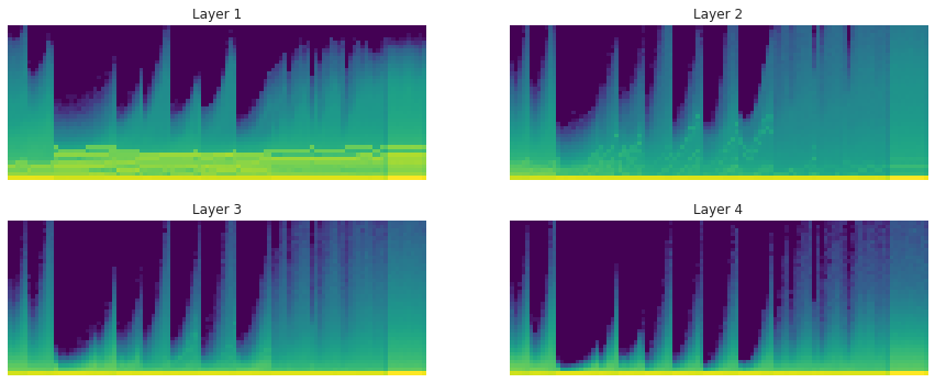
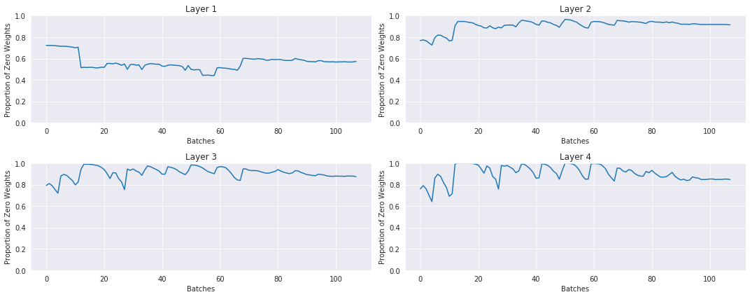
Let’s visualize the layers with the histograms like we did in the last lesson.
No LSUV, normal init: the histograms and proportions of non-zeros of the weights over time during training:
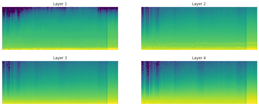
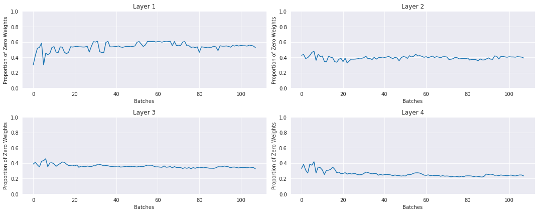
With LSUV: the histograms and proportions of non-zeros of the weights over time during training:
LSUV is something you run on all the layers at the beginning before starting training. You can also take more than one mini-batch.
Links, interesting forum posts:
Imagenette Dataset
We are getting great results very fast on MNIST. It’s time to put away MNIST and try a dataset that’s a bit harder. We aren’t quite ready to take on the ImageNet dataset, because ImageNet is very large and takes several days to train on one GPU. We need something that has a faster feedback loop than that for practising, learning, or researching.
Another image dataset is CIFAR-10, but this one consists of 32x32 images. It turns out that small images have very different characteristics to large images. Under 96x96 stuff behaves very differently. So stuff that works well on CIFAR-10, tends not to work well on larger images.
The same authors of the ‘All you need is a good init’ paper, Dmytro Mishkin et al., showed in another paper ‘Systematic evaluation of CNN advances on the ImageNet [2017]’ that:
… the use of 128x128 pixel images is sufficient to make qualitative conclusions about optimal network structure that hold for the full size Caffe and VGG nets. The results are obtained an order of magnitude faster than with the standard 224 pixel images.
If we do experiments with a dataset of 128x128 sized images the results will be applicable to larger images and we can save heap of time too. But simply resizing Imagenet down to 128x128 still takes too long because there are loads of different classes.
To fill this gap in the market, Jeremy has created Imagenette, which has normal sized images that are trainable in a sane amount of time. Imagenette consists of 3 datasets, which are all subsets of Imagenet.
- Imagenette: A subset of 10 easily classified classes from Imagenet.
- Imagewoof: A subset of 10 classes from Imagenet that aren’t easy to classify (all dog breeds).
- Image网 (or Imagewang): Imagenette and Imagewoof combined with some twists to make it into a tricky semi-supervised unbalanced classification problem.
Each of the datasets is available in 3 sizes:
- Full size.
- Shortest length resized to 160px (aspect ratio maintained).
- Shortest length resized to 320px (aspect ratio maintained).
Jeremy says…
A big part of a getting good at using deep learning in your domain is knowing how to create small, workable, useful datasets…
Try to come up with a toy problem or two that will give you insight into your full problem.
Data Block API Foundations
Imagenette isn’t big, but it’s too big to fit into RAM. We need to read it in one image at a time. We need to design and build fastai’s Data Block API from scratch.
What does the raw image data look like? Here is the directory structure of Imagenette and the number of images for each class:
imagenette2-160
├── train
│   ├── n01440764 [963 entries]
│   ├── n02102040 [955 entries]
│   ├── n02979186 [993 entries]
│   ├── n03000684 [858 entries]
│   ├── n03028079 [941 entries]
│   ├── n03394916 [956 entries]
│   ├── n03417042 [961 entries]
│   ├── n03425413 [931 entries]
│   ├── n03445777 [951 entries]
│   └── n03888257 [960 entries]
└── val
    ├── n01440764 [387 entries]
    ├── n02102040 [395 entries]
    ├── n02979186 [357 entries]
    ├── n03000684 [386 entries]
    ├── n03028079 [409 entries]
    ├── n03394916 [394 entries]
    ├── n03417042 [389 entries]
    ├── n03425413 [419 entries]
    ├── n03445777 [399 entries]
    └── n03888257 [390 entries]
There is are train and val directories. Each contains a subdirectory of JPEG images. The name of these subdirectories comes from Imagenet and is an encoding of the different categories and subcategories of objects. See the ImageNet explorer to get what I mean. The classes are all fairly balanced too.
All the images are roughly the same size, but have their own dimensions and are rectangular.
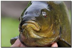
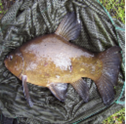
The first class n01440764 is a tench, which is a kind of fish:
What does the data of this image look like? If we read it into python with the image library PIL and convert it to a numpy array, we can see it is an array with shape (160, 237, 3) and its numbers look like:
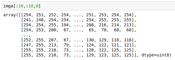
It’s an RGB image, with each pixel represented by 3 integers between 0 and 255, which say what colour the pixel is.
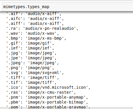
The first thing to build before the Datablack API is good way of grabbing all the files we need for training and validating our model. For image files, there are a number of different file types available. We can easily get a list of all the standard image file extensions from the python module mimetypes.
With the list of image file extensions we can do a walk through the dataset’s directory path to grab all these files. Here is the function used in fastai to recursively walk the directory path:
def get_files(path, extensions=None, recurse=False, include=None):
    path = Path(path)
    extensions = setify(extensions)
    extensions = {e.lower() for e in extensions}
    if recurse:
        res = []
        for i,(p,d,f) in enumerate(os.walk(path)):
            # returns (dirpath, dirnames, filenames)
            if include is not None and i==0:
                d[:] = [o for o in d if o in include]
            else:
                d[:] = [o for o in d if not o.startswith('.')]
            res += _get_files(p, f, extensions)
        return res
    else:
        f = [o.name for o in os.scandir(path) if o.is_file()]
        return _get_files(path, f, extensions)
Where the helper function _get_files takes a list of files in a directory and selects only the files that have the right extension. get_files also uses the fast low level file functions os.walk and os.scandir. These functions connect to library functions written in C and are orders of magnitudes faster than using something like python’s glob module.
DataBlock API Motivation
Why does FastAI have a DataBlock API? The API attempts to systematically define all the steps necessary to prepare data for a deep learning model, and create a mix and match rec ipe book for combining these steps.
To prepare for modeling, the following steps need to be performed:
- Get the source items
- Splitting the items into training and validation sets
- e.g. random fraction, folder name, CSV, …
- Labelling the items,
- e.g. from folder name, file name/re, CSV, …
- Processing the items (such as normalization)
- (Optional) Doing some Augmentation
- Transform items into tensors
- Make data into batches (
DataLoader) - (Optional) Transform per batch
- Combine the
DataLoaders together into aDataBunch - (Optional) Add a test set
Step 1 - ImageList
We need to get the source items and store them in some kind of collection data structure. We already created the ListContainer data structure for storing things in a list in a previous lecture that we can build upon here. What we want to do is not store the loaded source data in our list, rather store the filenames of the source data in a list and load things into memory when they are needed.
We create a base class called ItemList that has a get method, which subclasses override, and this get method should load and return what you put in there. An item is some data point, it could be an image, text sequence, whatever. For the case of the ImageList subclass, get will read the image file and return a PIL image object.
In summary, ItemList:
-
Is a list of items and a path where they came from
-
Optionally has a list of transforms, which are functions.
-
The list of transforms is
composedand applied every time yougetand item. So you get back a transformed item every time.
class ItemList(ListContainer):
    def __init__(self, items, path='.', tfms=None):
        super().__init__(items)
        self.path,self.tfms = Path(path),tfms

    def __repr__(self):
        return f'{super().__repr__()}\nPath: {self.path}'

    def new(self, items, cls=None):
        if cls is None: cls=self.__class__
        return cls(items, self.path, tfms=self.tfms)

    def  get(self, i): return i
    def _get(self, i): return compose(self.get(i), self.tfms)

    def __getitem__(self, idx):
        res = super().__getitem__(idx)
        if isinstance(res,list): return [self._get(o) for o in res]
        return self._get(res)
Aside: compose function: takes a list of functions and combines them into a pipeline that chains the outputs of the first function to input of the second and so on. In other words, a deep neural network is just a composition of functions (layers). NB, if you compose a list of functions then the order they are applied is right-to-left.
As a one-liner:
compose([f, g, h], x) = f(g(h(x)))
Here is the implementation for ImageList:
class ImageList(ItemList):
    @classmethod
    def from_files(cls, path, extensions=None, recurse=True, include=None, **kwargs):
        if extensions is None:
            extensions = image_extensions
        return cls(get_files(path, extensions, recurse=recurse, include=include), path, **kwargs)

    def get(self, fn):
        return PIL.Image.open(fn)
It defines the class method from_files to get a list of image files from a path. It uses the image_extensions and searches the path using our get_files function. Its get method is overridden and returns a PIL image object.
What about transforms? The first transform we create is make_rgb. When loading in images, if an image is grayscale then PIL will read it in as a rank 2 tensor, when we want it to be rank 3. So the make_rgb transform calls the PIL method to convert it to RGB:
def make_rgb(item):
    return item.convert('RGB')

il = ImageList.from_files(path, tfms=make_rgb)
Step 2 - Split Validation Set
Next we want to split the data into train and validation sets. For Imagenette training and validation sets have already been created for us and live in different directories. These are the train and val subdirectories. The path of an image in the dataset is something like this:
imagenette2-160/val/n02102040/n02102040_850.JPEG
The parent of the image is its label, and the parent of its parent (grandparent) denotes whether it is in the training or validation set. Therefore we will create a splitter function that splits on an image path’s grandparent:
def grandparent_splitter(fname, valid_name='valid', train_name='train'):
    gp = fname.parent.parent.name
    return True if gp==valid_name else False if gp==train_name else None
Let’s go further and encapsulate this into a SplitData class that can apply a splitter function to any kind of ItemList object:
class SplitData():
    def __init__(self, train, valid):
        self.train,self.valid = train,valid

    def __getattr__(self,k):
        # This is needed if we want to pickle SplitData and be able to load it back without recursion errors
        return getattr(self.train,k)

    def __setstate__(self,data:Any):
        self.__dict__.update(data)

    @classmethod
    def split_by_func(cls, il, f):
        lists = map(il.new, split_by_func(il.items, f))
        return cls(*lists)

    def __repr__(self):
        return f'{self.__class__.__name__}\nTrain: {self.train}\nValid: {self.valid}\n'
This has a split_by_func, which uses ItemList.new to coerce the train and test items back into their original ItemList type. So in the end we will get two ImageList objects for training and validation image sets.
This looks like this:
SplitData
  Train: ImageList (12894 items)
    [PosixPath('/home/ubuntu/.fastai/data/imagenette-160/train/n03888257/n03888257_9403.JPEG'),
     PosixPath('/home/ubuntu/.fastai/data/imagenette-160/train/n03888257/n03888257_6402.JPEG'),
     PosixPath('/home/ubuntu/.fastai/data/imagenette-160/train/n03888257/n03888257_4446.JPEG'),
     PosixPath('/home/ubuntu/.fastai/data/imagenette-160/train/n03888257/n03888257_13476.JPEG')...]
    Path: /home/ubuntu/.fastai/data/imagenette-160

  Valid: ImageList (500 items)
    [PosixPath('/home/ubuntu/.fastai/data/imagenette-160/val/n03888257/ILSVRC2012_val_00016387.JPEG'),
     PosixPath('/home/ubuntu/.fastai/data/imagenette-160/val/n03888257/ILSVRC2012_val_00034544.JPEG'),
     PosixPath('/home/ubuntu/.fastai/data/imagenette-160/val/n03888257/ILSVRC2012_val_00009593.JPEG'),
     PosixPath('/home/ubuntu/.fastai/data/imagenette-160/val/n03888257/ILSVRC2012_val_00020698.JPEG')...]
    Path: /home/ubuntu/.fastai/data/imagenette-160
Step 3 - Labelling
Labelling is a little more tricky because it has to be done after splitting, at it uses training set information to apply to the validation set. To do this we need to create something called a Processor. For example, we could have a processor whose job it was to encoded the label strings into numbers:
- “tench” => 0
- “french horn” => 1
We would need the training set to have the same mapping as the validation set. So we need to create a vocabulary which encodes our classes to numbers and tells us the order they are in. We create this vocabulary from the training set and use that to transform the training and the validation sets.
Other examples of processors would be processing texts to tokenize and numericalize them. Text in the validation set should be numericalized the same way as the training set. Or in another case with tabular data, where we wish to fill missing values with, for instance, the median computed on the training set. The median is stored in the inner state of the Processor and applied on the validation set.
Here we label according to the folders of the images, so simply fn.parent.name. We label the training set first with a newly created CategoryProcessor so that it computes its inner vocab on that set. Then we label the validation set using the same processor, which means it uses the same vocab.
class Processor():
    def process(self, items): return items

class CategoryProcessor(Processor):
    def __init__(self): self.vocab=None

    def __call__(self, items):
        #The vocab is defined on the first use.
        if self.vocab is None:
            self.vocab = uniqueify(items)
            self.otoi  = {v:k for k,v in enumerate(self.vocab)}
        return [self.proc_(o) for o in items]
    def proc_(self, item):  return self.otoi[item]

    def deprocess(self, idxs):
        assert self.vocab is not None
        return [self.deproc_(idx) for idx in idxs]
    def deproc_(self, idx): return self.vocab[idx]
def label_by_func(sd, f, proc_x=None, proc_y=None):
    train = LabeledData.label_by_func(sd.train, f, proc_x=proc_x, proc_y=proc_y)
    valid = LabeledData.label_by_func(sd.valid, f, proc_x=proc_x, proc_y=proc_y)
    return SplitData(train,valid)


ll = label_by_func(sd, parent_labeler, proc_y=CategoryProcessor())
LabeledData is an object that has two ItemList objects: x and y. In this case x is an ImageList (basically a list of file paths) and y is a ItemList (a generic container, here it contains labels: 0, 1, etc).
This output ll looks like:
SplitData
 Train: LabeledData
  x: ImageList (12894 items)
  [...]
  Path: ...
  y: ItemList (12894 items)
  [0,0,0,0,0,0...]
  Path: ...

 Valid: LabeledData
  x: ImageList (500 items)
  [...]
  Path: ...
  y: ItemList (500 items)
  [0,0,0,0,0,0...]
  Path: ...
Question: How do could we handle unseen labels?
You could group together rare labels into a single label called ‘other’/’unknown’
Step 4 - DataBunch
A DataBunch has a training dataloader and a validation data loader. Here is the class:
class DataBunch():
    def __init__(self, train_dl, valid_dl, c_in=None, c_out=None):
        self.train_dl,self.valid_dl,self.c_in,self.c_out = train_dl,valid_dl,c_in,c_out

    @property
    def train_ds(self): return self.train_dl.dataset

    @property
    def valid_ds(self): return self.valid_dl.dataset


def databunchify(sd: SplitData, bs: int, c_in=None, c_out=None, **kwargs):
    dls = get_dls(sd.train, sd.valid, bs, **kwargs)
    return DataBunch(*dls, c_in=c_in, c_out=c_out)

SplitData.to_databunch = databunchify
All the steps
Here’s the fully dataloading pipeline using the Data Block API: grab the path, untar the data, list the transforms, get item list, split the data, label the data, create a databunch.
path = datasets.untar_data(datasets.URLs.IMAGENETTE_160)
tfms = [make_rgb, ResizeFixed(128), to_byte_tensor, to_float_tensor]

il = ImageList.from_files(path, tfms=tfms)
sd = SplitData.split_by_func(il, partial(grandparent_splitter, valid_name='val'))
ll = label_by_func(sd, parent_labeler, proc_y=CategoryProcessor())
data = ll.to_databunch(bs, c_in=3, c_out=10, num_workers=4)
New CNN Model
Let’s train a CNN using our databunch.
Get the callbacks:
cbfs = [partial(AvgStatsCallback,accuracy),
        CudaCallback]
Next we need to normalize all the images for training. With colour images we need to normalize all three channels so we need means and standard deviations for each of channels. We can get these statistics from a batch/batches from the training set.
def normalize_chan(x, mean, std):
    return (x-mean[...,None,None]) / std[...,None,None]

_m = tensor([0.47, 0.48, 0.45])
_s = tensor([0.29, 0.28, 0.30])
norm_imagenette = partial(normalize_chan, mean=_m.cuda(), std=_s.cuda())

cbfs.append(partial(BatchTransformXCallback, norm_imagenette))
We build our model using Bag of Tricks for Image Classification with Convolutional Neural Networks, in particular: we don’t use a big conv 7x7 at first but three 3x3 convs, and don’t go directly from 3 channels to 64 but progressively add those. The first 3 layers are very important. Back in the old days people would use 5x5 and 7x7 kernels for the first layer. However the Bag of Tricks paper shows that this isn’t a good idea, which refers to many previous citations and competition winning models. The message is clear - 3x3 kernels give you more bang for your buck. You get deeper, you get the same receptive field, and it’s also faster because you have less working going on. The 7x7 conv layer also is over 5 times slower than a single 3x3 as well.
(Recall - a conv_layer composes a Conv2d, Generalized ReLU, and a normalization (e.g. batchnorm))
The first layer is a 3x3 kernel and a known number of channels data.c_in, which in this case is 3 (RGB). What about the number of outputs? The kernel has 9*c_in numbers. We want to make sure that our kernal has something useful to do. You don’t want more numbers coming out than are coming in, because its a waste of time. We set the number of outputs to the closest power of 2 below 9*c_in. (For 9*3 that is 16). The stride of the first layer is also 1, so the first layer doesn’t downsample.
Then for the next two layers we successively mutiply the number of outputs by 2 and set stride to 2.
(Anywhere you see something that isn’t a 3x3 kernel - have a big think as to whether it makes sense.)
We use 4 conv_layers in the body of the model with sizes: nfs = [64,64,128,256]
Here is the code for the model:
import math
def prev_pow_2(x): return 2**math.floor(math.log2(x))

def get_cnn_layers(data, nfs, layer, **kwargs):
    def f(ni, nf, stride=2): return layer(ni, nf, 3, stride=stride, **kwargs)
    l1 = data.c_in
    l2 = prev_pow_2(l1*3*3)
    layers =  [f(l1  , l2  , stride=1),
               f(l2  , l2*2, stride=2),
               f(l2*2, l2*4, stride=2)]
    nfs = [l2*4] + nfs
    layers += [f(nfs[i], nfs[i+1]) for i in range(len(nfs)-1)]
    layers += [nn.AdaptiveAvgPool2d(1), Lambda(flatten),
               nn.Linear(nfs[-1], data.c_out)]
    return layers

def get_cnn_model(data, nfs, layer, **kwargs):
    return nn.Sequential(*get_cnn_layers(data, nfs, layer, **kwargs))
We run this with cosine 1cycle annealing:
sched = combine_scheds([0.3,0.7], cos_1cycle_anneal(0.1,0.3,0.05))

learn,run = get_learn_run(nfs, data, 0.2, conv_layer, cbs=cbfs+[
    partial(ParamScheduler, 'lr', sched)
])
This gives performance 72.6% for Imagenette, which is not bad and on the right track.
Universal Optimizer
Every other deep learning library treats every optimizer algorithm as a totally different object. But this is an artificial categorization - there is however only one optimizer and lots of stuff you can add to it.
We are going to implement this paper: Large Batch Optimization for Deep Learning: Training BERT in 76 minutes. We will implement this equation set from the paper:
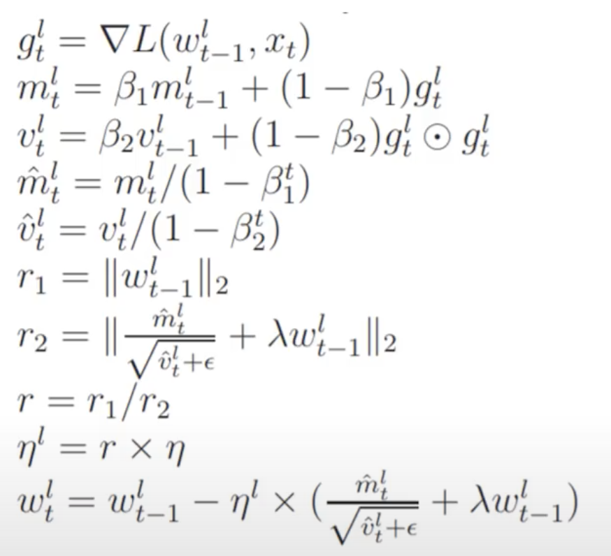
This looks scary because of the mathematical notation and greek symbols, but we will find when we turn it into code it is actually very simple. All these terms are separable parts or ‘steppers’ of a more general optimizer class.
All experiments will be done with our CNN model using the Imagenette dataset.
The Optimizer Class
Let’s build own Optimizer class. It needs to have a zero_grad method to set the gradients of the parameters to zero and a step method that does some kind of step. The thing we will do differently from all other libraries is that the functionality of step will be abstracted out into a composition of stepper functions. The Optimizer class will simply have a list of steppers to iterate through.
In order to optimize something we need to know what all the parameter tensors are in a model. However we might want to say: “the last two layers should have a different learning rate to the rest of the layers.” We can instead decide group different parameters into param_groups, which would basically be a list of lists. Each parameter group can have its own set of hyperparameters (e.g. learning rate, weight decay, etc) and each parameter group will have its own dictionary to store these hyperparameters.
Code for the Optimizer class, with a way of getting default hyperparameters for the steppers:
class Optimizer():
    def __init__(self, params, steppers, **defaults):
        self.steppers = listify(steppers)
        maybe_update(self.steppers, defaults, get_defaults)
        # might be a generator
        self.param_groups = list(params)
        # ensure params is a list of lists
        if not isinstance(self.param_groups[0], list): self.param_groups = [self.param_groups]
        self.hypers = [{**defaults} for p in self.param_groups]

    def grad_params(self):
        # return flattened list of parameters from all layers
        return [(p,hyper) for pg,hyper in zip(self.param_groups,self.hypers)
            for p in pg if p.grad is not None]

    def zero_grad(self):
        for p,hyper in self.grad_params():
            p.grad.detach_()
            p.grad.zero_()

    def step(self):
        for p,hyper in self.grad_params(): compose(p, self.steppers, **hyper)


def maybe_update(os, dest, f):
    for o in os:
        for k,v in f(o).items():
            if k not in dest: dest[k] = v

def get_defaults(d): return getattr(d,'_defaults',{})
This is basically the gist of PyTorch’s optim.Optimizer, but with the steppers. A stepper is a function that forms part of the optimizer recipe. An example of stepper is sgd_step:
def sgd_step(p, lr, **kwargs):
  """
  SGD step
  p : parameters
  lr : learning rate
  """
	p.data.add_(-lr, p.grad.data)
	return p
In other words we can create an optimizers like this:
opt_func = partial(Optimizer, steppers=[sgd_step])
When we call step, it loops through all our parameters and composes all our steppers then calls that composition on the parameters.
Weight Decay
(This subsection is combines explanations from the 09_optimizers.ipynb notebook and this fastai blog post)
By letting our model learn high parameters, it might fit all the data points in the training set with an over-complex function that has very sharp changes, which will lead to overfitting.
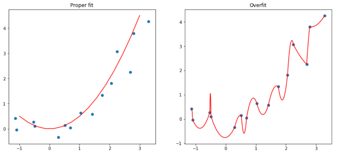
Weight decay comes from the idea of L2 regularization, which consists in adding to your loss function the sum of all the weights squared. Why do that? Because when we compute the gradients, it will add a contribution to them that will encourage the weights to be as small as possible.
Classic L2 regularization consists of adding the sum of all the weights squared to the loss multiplied by a hyperparameter, wd. The intuition is that large weight values get ‘exploded’ when they are squared which will contribute to a much larger loss. The optimizer will therefore shy away from such regions of parameter space. In theory, this would be like adding this big sum to the total loss at the end of the forward pass:
loss_with_wd = loss + wd * all_weights.pow(2).sum() / 2
This is never how this is implemented in practice however. The sum would require a massive reduction of all the weight tensors at every update step, which would be expensive and potentially numerically unstable (more so with lower precision). We only need the derivative of that wrt to each of the weights, and remembering that $\frac{\partial}{\partial w_j} \sum_i w_i^2 = 2 w_j$, you can see that adding the big sum to the loss is equivalent to locally updating the gradients of the parameters like so:
weight.grad += wd * weight
For the case of vanilla SGD this is equivalent to updating the parameters with:
weight = weight - lr * (weight.grad + wd.weight)
This technique is called weight decay, as each weight is decayed by a factor lr * wd, as it’s shown in this last formula.
This is a slightly confusing thing - Aren’t L2 regularization and Weight decay the same thing? – Not exactly. Only in the case of vanilla SGD are they the same.
For algorithms such as momentum, RMSProp, and Adam, the update has some additional formulas around the gradient. For SGD with momentum the formula is:
moving_avg = alpha * moving_avg + (1 - alpha) * w.grad
w = w - lr * moving_avg
If we did L2 regularization this would become:
moving_avg = alpha * moving_avg + (1 - alpha) * (w.grad + wd*w)
w = w - lr * moving_avg
Whereas with weight decay it would be:
moving_avg = alpha * moving_avg + (1 - alpha) * w.grad
w = w - lr * moving_avg - lr * wd * w
We can see that the part subtracted from w linked to regularization isn’t the same in the two methods, and the wd is polluted by the (1-alpha) factor. When using something more complicated like the Adam optimizer, it gets even more polluted. Most libraries use the first formulation, but as it was pointed out in Decoupled Weight Regularization by Ilya Loshchilov and Frank Hutter, it is better to use the second one with the Adam optimizer, which is why the fastai library made it its default. This implemation of Adam and decoupled weight decay is often called AdamW.
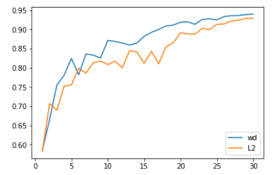
The above is a comparison between the two done by Jeremy and Sylvain. The weight decay formulation gives slightly better results.
Weight decay is also super simple to implement too - you simply subtract lr*wd*weight from the weights before the optimizer step. We could create some abstract base class for stepper or just use a function in python:
def weight_decay(p, lr, wd, **kwargs):
    p.data.mul_(1 - lr*wd)
    return p

weight_decay._defaults = dict(wd=0.)
In python you can attach an attribute to any object in python including functions. Here we attach a dictionary _defaults for default hyper-parameter values. Alternatively, if you were using an abstract base class you would just have a class attribute _defaults to get the sam effect.
Similarly, if you wanted to use L2 regularization then the implementation is also simply - add wd*weight to the gradients:
def l2_reg(p, lr, wd, **kwargs):
    p.grad.data.add_(wd, p.data) # add is actually scaled-add
    return p

l2_reg._defaults = dict(wd=0.)
Momentum
Momentum will require an optimizers that has some state because it needs to remember what it did in the last update to do the current update.
Momentum requires to add some state. We need to save the moving average of the gradients to be able to do the step and store this inside the optimizer state. We need to track, for every single parameter, what happened last time. This is actually quite a bit of state - if you had 10 million activations in your network, you now have 10 million more floats that you have to store.
To implement this we need to create a new subclass of Optimizer which maintains a state attribute which can store running Stats of things, which are updated every step. A Stat is an object that has two methods and an attribute:
init_state, that returns the initial state (a tensor of 0. for the moving average of gradients)-
update, that updates the state with the new gradient value. Takes a state dict and returns an updated state dict. - We also read the
_defaultsvalues of those objects, to allow them to provide default values to hyper-parameters.
The StatefulOptimizer:
class StatefulOptimizer(Optimizer):
    def __init__(self, params, steppers, stats=None, **defaults):
      	self.stats = listify(stats)
        maybe_update(self.stats, defaults, get_defaults)
        super().__init__(params, steppers, **defaults)
        self.state = {}

    def step(self):
      	for p,hyper in self.grad_params():
            if p not in self.state:
                # Create a state for p and
                # call all the statistics to initalize it
                self.state[p] = {}
                maybe_update(self.stats, self.state[p], lambda o: o.init_state(p))
            state = self.state[p]
            for stat in self.stats:
                state = stat.update(p, state, **hyper)

            # run the steppers
            compose(p, self.steppers, **state, **hyper)
            self.state[p] = state
For momentum we are mainting an moving average of the parameter gradients. The Stat for this would be:
class AverageGrad(Stat):
    # with NO dampening
    _defaults = dict(mom=0.9)

    def init_state(self, p):
        return {"grad_avg": torch.zeros_like(p.grad.data)}

    def update(self, p, state, mom, **kwargs):
        state["grad_avg"].mul_(mom).add_(p.grad.data)
        return state
With this we can now implement MomentumSGD a new stepper, momentum_step:
def momentum_step(p, lr, grad_avg, **kwargs):
    p.add_(-lr, grad_avg)
    return p


sgd_mom_opt = partial(StatefulOptimizer,
                      steppers=[momentum_step,
                                weight_decay],
                      stats=AverageGrad(), wd=0.01)
Aside: Python’s Wonderful kwargs
One of the features of python that makes this work is the wonderfully flexible way that python handles parameters and lists of keyword arguments. All the different stepper functions take a weight tensor plus some individual set of positional arguments. It would be complicated as hell trying to call a list of stepper functions with a list of which of all their positional arguments. However if you stick on a **kwargs to a stepper’s parameter list then it enables you to throw a dictionary of all the parameters name/value pairs to all the stepper functions, and when it comes time to call the stepper it will simply take what it needs from kwargs and ignore everything else!
This trivial example shows what I mean:
def foo(bar, lol, baz, **kwargs):
    print(bar, lol, baz)

def boo(biz, **kwargs):
    print(biz)

params = {"lol": 2, "baz": 3, "biz": 5}
foo(1, **params)
boo(**params)

## This outputs:
## 1 2 3
## 5
params has all of the kwargs for all of the functions. Functions foo and boo only take what they need from params. The only thing you need to be careful of here is that you don’t have any stepper functions whose parameters share the same name, but are semantically different things. You could perhaps have a check on params to throw and exception if a key is overwritten to prevent this silent bug.
Weight Decay + Batch Norm: A Surprising Result
Weight decay scales the weights by a factor of (1-wd), however batch norm is invariant to weight scaling, so weight decay followed by batch norm effectively undoes the weight decay.
This was pointed out in the paper: L2 Regularization versus Batch and Weight Normalization.
Empirically, however, it has been found that weight decay and batch norm is actually anyway better than batch norm and no weight decay. This blog post explores this for vanillia SGD:
…without an L2 penalty or other constraint on weight scale, introducing batch norm will introduce a large decay in the effective learning rate over time. But an L2 penalty counters this.
This paper - Three Mechanisms of Weight Decay Regularization - identifies three different ways weight decay exerts a regularization effect, depending on the different optimization algorithm and architecture.
In reality, we don’t really know why weight decay works, but empirically it seems to help and basically all models use it. :-)
Momentum Experiments
Momentum is also interesting, and we really don’t understand it works.
Let’s create some fake data series of 200 normally distributed points and plot the moving average of this series with different beta values: [0.5, 0.7, 0.9, 0.99]
The regular momentum:
def mom1(avg, beta, yi, i):
    if avg is None: avg=yi
    res = beta*avg + yi
    return res
Here is a plot of the data (blue) and moving average (red):
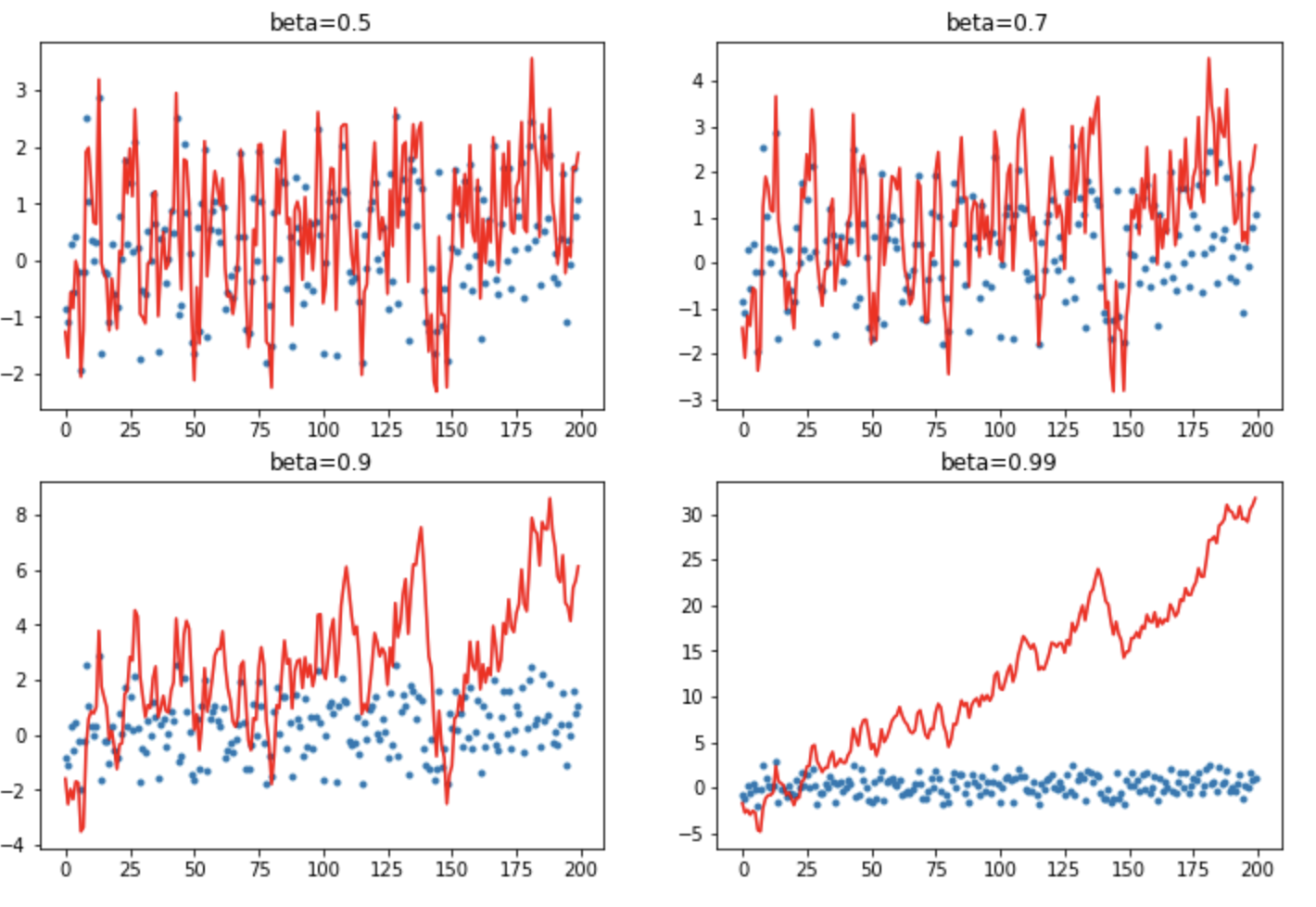
With very little momentum (small beta) it is very bumpy/highly variant. When you get up to larger values of momentum it shoots off and the new values its seeing can’t slow it down. So you have to be really careful when it comes to high momentum values.
This is a rather naive implementation. We can fix it by instead using a Exponentially Weighted Moving Average (or EWMA, also called lerp in PyTorch):
def ewma(v1, v2, beta):
    return beta*v1 + (1-beta)*v2

def mom2(avg, beta, yi, i):
    if avg is None: avg=yi
    avg = ewma(avg, yi, beta)
    return avg
This helps to dampen the incoming data point which stops it being so bumpy for lower momentum values. . Plotting the same again:
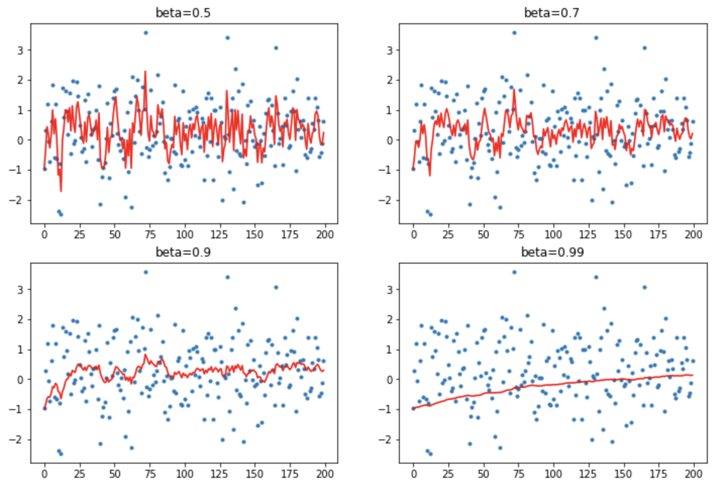
This works much better. So we’re done? - Not quite.
What if the thing we are trying to match isn’t just random, but is some function like a polynomial. We’ve also added an outlier at the start.
def lin_comb(v1, v2, beta):
    return beta*v1 + (1-beta)*v2

def mom2(avg, beta, yi, i):
    if avg is None: avg=yi
    avg = lin_comb(avg, yi, beta)
    return avg
Let’s see how EWMA does here:
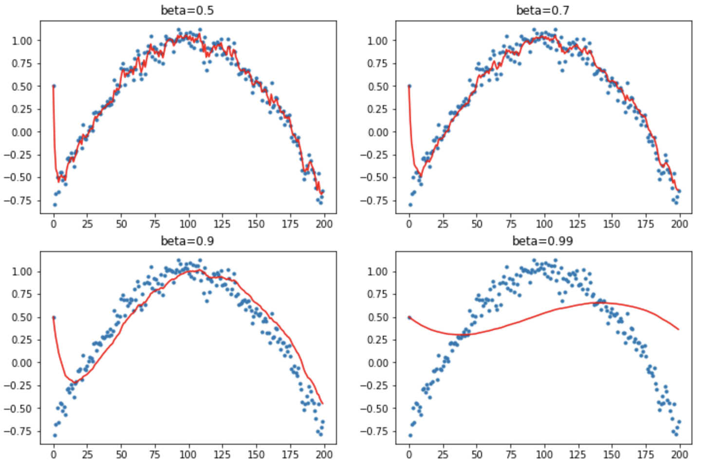
The outlier at the start causes trouble with the higher momentum values. The first item is massively biasing the start.
We need to do something called Debiasing (aka bias correction). We want to make sure that no observation is weighted too highly. Normal way of doing EWMA gives the first point far too much weight. These first points are all zero, so the running averages are all biased low. Add a correction factor dbias: $x_i = x_i/(1 - \beta^{i+1})$. When $i$ is large this correction factor tends to 1 - it only pushes up the initial values.
def mom3(avg, beta, yi, i):
    if avg is None: avg=0
    avg = lin_comb(avg, yi, beta)
    return avg/(1-beta**(i+1)
Plot that:
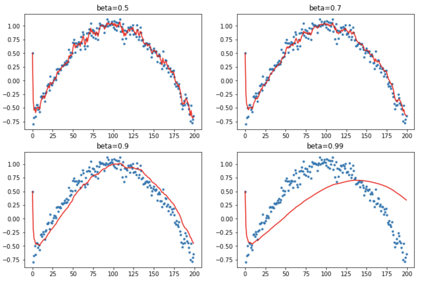
This is pretty good. It debiases pretty well even if we have a bad starting point. You can see why beta=0.9 is a popular value.
Adam Algorithm
Let’s use what we’ve learned to implement the optimizer Adam. The algorithm definition from the Adam paper (2014) is:
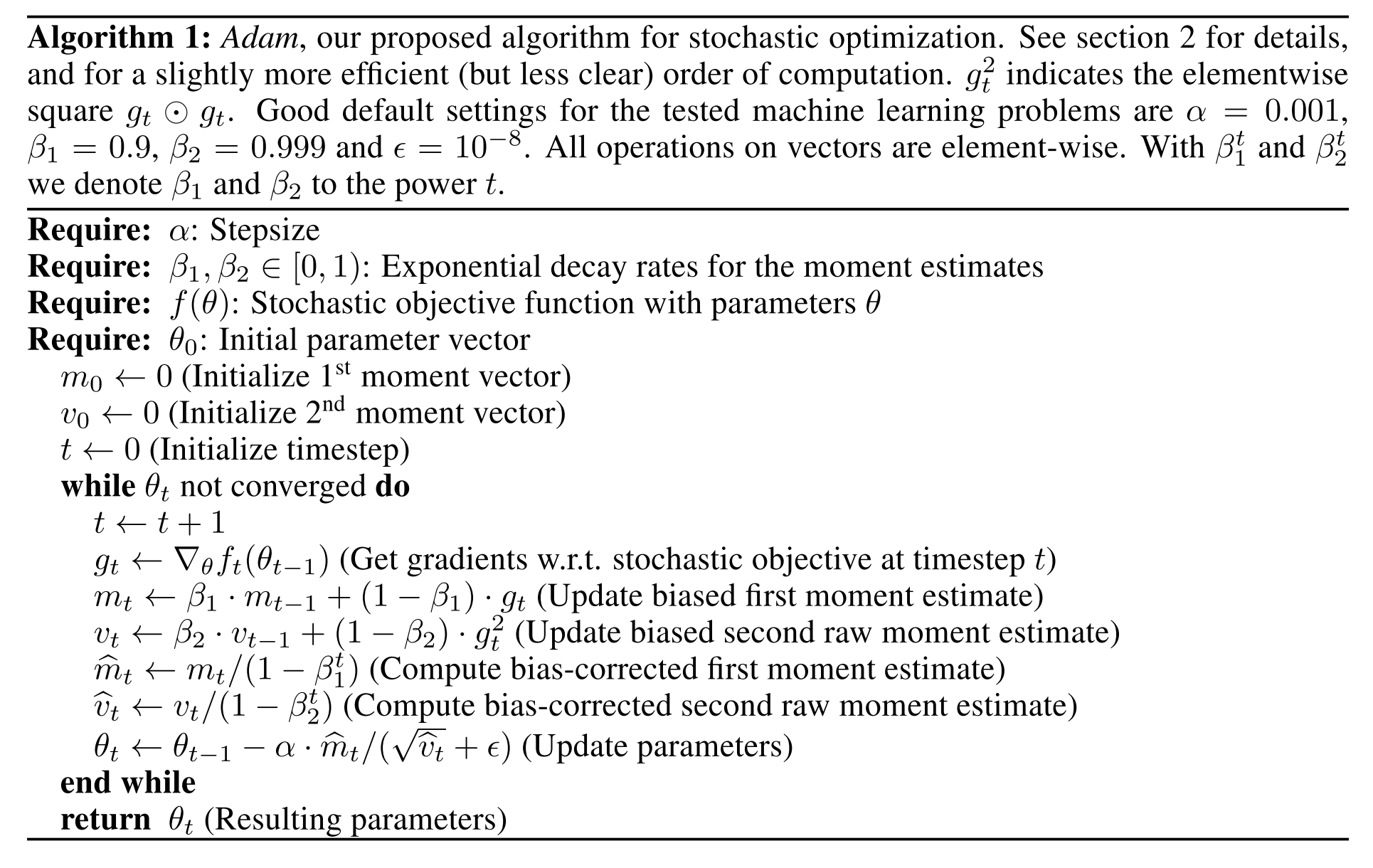
If we look inside the while loop, and stare at the maths there is nothing in there we haven’t seen already. $g$ is the gradients of the weights, $m$ is the EWMA of the gradients, and $v$ is the EMWA of the square of the gradients. $m$ and $v$ are then debiased, as we have seen above.
Adam is just dampened debiased momentum divided by dampened debiased root sum of squared gradients.
To implement Adam we will need to implement the following:
- EWMA of the gradients - a
Statsubclass. - EWMA of the square of the gradients - a
Statsubclass. - A debiasing function. This will need to know which step we are on.
- A step counter - a
Statsubclass
class AverageGrad(Stat):
    _defaults = dict(mom=0.9)

    def __init__(self, dampening:bool=False):
        self.dampening = dampening

    def init_state(self, p):
        return {'grad_avg': torch.zeros_like(p.grad.data)}

    def update(self, p, state, mom, **kwargs):
        state['mom_damp'] = 1 - mom if self.dampening else 1.
        state['grad_avg'].mul_(mom).add_(state['mom_damp'], p.grad.data)
        return state


class AverageSqrGrad(Stat):
    _defaults = dict(sqr_mom=0.99)

    def __init__(self, dampening:bool=False):
        self.dampening = dampening

    def init_state(self, p):
        return {'sqr_avg': torch.zeros_like(p.grad.data)}

    def update(self, p, state, sqr_mom, **kwargs):
        state['sqr_damp'] = 1 - sqr_mom if self.dampening else 1.
        state['sqr_avg'].mul_(sqr_mom).addcmul_(state['sqr_damp'],
                                                p.grad.data,
                                                sp.grad.data)
        return state


class StepCount(Stat):
    def init_state(self, p): return {'step': 0}

    def update(self, p, state, **kwargs):
        state['step'] += 1
        return state


def debias_term(mom, damp, step):
    # if we don't use dampening (damp=1) we need to divide by 1-mom because
    # that term is missing everywhere
    return damp * (1 - mom**step) / (1-mom)
Adam as a stepper is now:
def adam_step(p, lr, mom, mom_damp, step, sqr_mom, sqr_damp, grad_avg, sqr_avg, eps, **kwargs):
    debias1 = debias_term(mom, mom_damp, step)
    debias2 = debias_term(sqr_mom, sqr_damp, step)
    p.data.addcdiv_(-lr / debias1,
                    grad_avg,
                    (sqr_avg/debias2).sqrt() + eps)
adam_step._defaults = dict(eps=1e-5)


def adam_opt(xtra_step=None, **kwargs):
    return partial(StatefulOptimizer,
                   steppers=[adam_step,weight_decay]+listify(xtra_step),
                   stats=[AverageGrad(dampening=True),
                          AverageSqrGrad(),
                          StepCount()],
                   **kwargs)
Note that the weight decay and Adam step are totally decoupled. This is an implemention the AdamW algorithm, mentioned above in the weight decay subsection. First you decay the weights, then you do the Adam step.
The epsilon eps in Adam is super important to think about. What if we set eps=1? Most of the time the gradients are going to be smaller than 1 and the squared gradients are going to be much smaller than 1. So eps=1 is going to be much bigger than (sqr_avg/debias2).sqrt(), so eps will dominate and the optimizer will be pretty close to being SGD with debiased-dampened momentum.
Whereas, if eps=1e-7 then we are really using the (sqr_avg/debias2).sqrt() term. If you have some activation that has had a very small squared gradients for a while, the value of this term could well be 1e-6. Dividing by this is equivalent to multiplying by a million, which would kill your optimizer. The trick getting Adam and friends working well is a value between eps=1e-3 and eps=1e-1.
Most people use 1e-7, which is equivalent to multiplying by 10 million. Here eps is basically just a small hack number put in to avoid a possible division by zero. We can instead treat eps as a kind of smoothing factor that enables the optimizer to behave more like momentum SGD sometimes and normal Adam at other times.
LAMB Algorithm
It’s then super easy to implement a new optimizer. This is LAMB from a very recent paper (2019):
\[\begin{align} g_{t}^{l} &= \nabla L(w_{t-1}^{l}, x_{t}) \\ m_{t}^{l} &= \beta_{1} m_{t-1}^{l} + (1-\beta_{1}) g_{t}^{l} \\ v_{t}^{l} &= \beta_{2} v_{t-1}^{l} + (1-\beta_{2}) g_{t}^{l} \odot g_{t}^{l} \\ m_{t}^{l} &= m_{t}^{l} / (1 - \beta_{1}^{t}) \\ v_{t}^{l} &= v_{t}^{l} / (1 - \beta_{2}^{t}) \\ r_{1} &= \|w_{t-1}^{l}\|_{2} \\ s_{t}^{l} &= \frac{m_{t}^{l}}{\sqrt{v_{t}^{l}} + \epsilon} + \lambda w_{t-1}^{l} \\ r_{2} &= \| s_{t}^{l} \|_{2} \\ \eta^{l} &= \eta * r_{1}/r_{2} \\ w_{t}^{l} &= w_{t-1}^{l} - \eta_{l} * s_{t}^{l} \\ \end{align}\]This is stuff we’ve seen before in Adam plus a few extras:
- $m$ and $v$ are the debiased dampened momentum and the debiased dampened square of the gradients exactly like Adam.
- $|w^l_{t-1}|_2$ is the layerwise l2-norm of the weights in layer $l$.
- The learning rate $\eta^l$ is adapted individually for every layer.
- It requires the same amount of state as Adam.
As code:
def lamb_step(p, lr, mom, mom_damp, step,
              sqr_mom, sqr_damp, grad_avg,
              sqr_avg, eps, wd, **kwargs):
    debias1 = debias(mom,     mom_damp, step)
    debias2 = debias(sqr_mom, sqr_damp, step)

    r1 = p.data.pow(2).mean().sqrt()  # layerwise L2 norm

    step = (grad_avg/debias1)/((sqr_avg/debias2).sqrt()+eps) + wd*p.data

    r2 = step.pow(2).mean().sqrt()	# layerwise L2

    p.data.add_(-lr * min(r1/r2,10), step)
    return p

lamb_step._defaults = dict(eps=1e-6, wd=0.)


def lamb_opt(**kwargs):
    return partial(StatefulOptimizer,
                   steppers=lamb_step,
                   stats=[AverageGrad(dampening=True),
                          AverageSqrGrad(),
                          StepCount()],
                   **kwargs)
The ratio r1/r2 is called the ‘trust ratio’ by the original authors. In most implementations this trust ratio’s upper value is clipped to make LAMB more stable. This upper bound is typically set to 10 or 100.
Data Augmentation
Up to this point we have created our datablocks API and optimizers and we have these running nicely together in a Learner class (which replaces the Runner class seen in prior lessons). With this we can train a reasonably good Imagenette model with a CNN (09b_learner.ipynb). But Imagenette is a bit short of data, so to make an even better model we should use data augmentation.
It’s important when doing data augmentation to look at or listen to or understand your augmented data to make sure the new data is of good enough quality and it representative of the original data. Don’t just chuck it into a model and hope for the best. Let’s look at an example where this can create problems with resizing images.
Resizing
Let’s load up some imagenette:
path = datasets.untar_data(datasets.URLs.IMAGENETTE)
tfms = [make_rgb, ResizeFixed(128), to_byte_tensor, to_float_tensor]

def get_il(tfms):
    return ImageList.from_files(path, tfms=tfms)

il = get_il(tfms)
Our transforms here are:
- Convert image to RGB
- Resize to 128x128
- Convert from Pillow object (bytes) to byte tensor
- Convert to float tensor
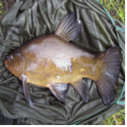
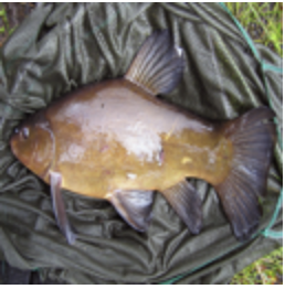
Here is an image from the tench class with the ResizeFixed(128) transform:
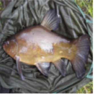
However, here is what the original looks like:
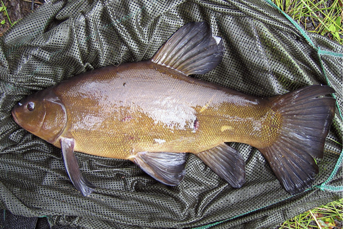
Notice how the fish’s scale texture and the texture of the net is completely lost during the resizing. This resizing method may be chucking out useful textures that are key to identifying certain classes. Be careful of resampling methods, you can quickly lose some textures!
(Perhaps one could try making the resampling method used in a resizing random as a method of data augmentation?)
There are many resampling methods. Be critical about the resizing. Look at the augmented data and make sure that you aren’t losing key information like textures. Pillow has many different resizing methods. They recommend ANTIALIAS as a good default. Let’s look at the different resampling methods offered by Pillow:
 ANTIALIAS |
 BICUBIC |
|---|---|
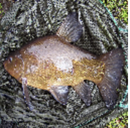 NEAREST |
 BICUBIC/NEAREST |
NEAREST is the only one that preserves the textures. There are a lot of aliasing artifacts however. The last one, BICUBLIC/NEAREST, does a resize to 256x256 with BICUBIC then another resize to 128x128 with NEAREST to achieve a pretty good compromise.
Topical: This recent tweet shows the difference between image resize methods in tensorflow and pytorch. “Something to check when porting and comparing models between frameworks”
Flipping, Rotating, Cropping
Flipping is a great data augmentation for vision. A very important point to make here is that doing image transforms on bytes is much faster than doing them on floats, because bytes are 4 times smaller than floats. If you are flipping an image, flipping bytes is identical to flipping floats in terms of the outcome. You should definitely everything you can while your image is still bytes (a Pillow object). However you should be careful when doing destructive transformations on bytes, because you can get rounding errors and saturation errors. Again - inspect the steps and take nothing for granted.
Flip:
class PilRandomFlip(PilTransform):
    def __init__(self, p=0.5): self.p=p
    def __call__(self, x):
        return x.transpose(PIL.Image.FLIP_LEFT_RIGHT) if random.random()<self.p else x
It’s therefore really important to think when in your transformation pipeline you do certain image transforms.
We can easily extend this to doing the whole dihedral group of transformations (random horizontal flip, random vertical flip, and the four 90 degrees rotations) by passing a int between 0 and 6 to transpose:
class PilRandomDihedral(PilTransform):
    def __init__(self, p=0.75):
        self.p=p*7/8 #Little hack to get the 1/8 identity dihedral transform taken into account.
    def __call__(self, x):
        if random.random()>self.p: return x
        return x.transpose(random.randint(0,6))
We can also do random cropping. A great way to do data augmentation is to grab a small piece of an image and zoom into that piece. We can do this by randomly cropping and then down sizing the selection.
Naively we can do this with two steps in Pillow - crop and resize:
img.crop((60,60,320,320)).resize((128,128), resample=PIL.Image.BILINEAR)
However this degrades quality. You can instead do it all in one step with Pillow’s transform:
img.transform((128,128), PIL.Image.EXTENT, cnr2, resample=resample)
This is an example of doing multiple destructive transformations when the image is still in bytes. Do them all in one go, if possible, or wait until they are floats.
RandomResizeCrop the usual data augmentation used on ImageNet (introduced here) that consists of selecting 8 to 100% of the image area and a scale between 3/4 and 4/3 as a crop, then resizing it to the desired size. It combines some zoom and a bit of squishing at a very low computational cost.
class RandomResizedCrop(GeneralCrop):
    def __init__(self, size, scale=(0.08,1.0), ratio=(3./4., 4./3.), resample=PIL.Image.BILINEAR):
        super().__init__(size, resample=resample)
        self.scale,self.ratio = scale,ratio

    def get_corners(self, w, h, wc, hc):
        area = w*h
        #Tries 10 times to get a proper crop inside the image.
        for attempt in range(10):
            area = random.uniform(*self.scale) * area
            ratio = math.exp(random.uniform(math.log(self.ratio[0]), math.log(self.ratio[1])))
            new_w = int(round(math.sqrt(area * ratio)))
            new_h = int(round(math.sqrt(area / ratio)))
            if new_w <= w and new_h <= h:
                left = random.randint(0, w - new_w)
                top  = random.randint(0, h - new_h)
                return (left, top, left + new_w, top + new_h)

        # Fallback to squish
        if   w/h < self.ratio[0]: size = (w, int(w/self.ratio[0]))
        elif w/h > self.ratio[1]: size = (int(h*self.ratio[1]), h)
        else:                     size = (w, h)
        return ((w-size[0])//2, (h-size[1])//2, (w+size[0])//2, (h+size[1])//2)
Jeremy says…
The most useful transformation by far shown in competition winners, is to grab a small piece of the image of the image and zoom into it. This is called a random resize crop. This is also really useful to know in any domain. For example, in NLP a really useful thing to do is a grab different sized chunks of contiguous text. With audio, if you are doing speech recognition, grab different sized pieces of the utterances. If you can find a way to get different slices of your data, it’s a fantastically useful data augmentation approach. So this is by far the most important augmentation in every imagenet winner in the last 6 years or so.
Perspective Transform
What RandomResizeCrop does, however, is it squishes the aspect ratio to some between 3:4 and 4:3. This can distort the image making objects expand outwards and inwards. Probably what they really want to do is something physically reasonable. If you are above or below something then your perspective changes. What would be even better is perspective warping.
To do perspective warping, we map the corners of the image to new points: for instance, if we want to tilt the image so that the top looks closer to us, the top/left corner needs to be shifted to the right and the top/right to the left. To avoid squishing, the bottom/left corner needs to be shifted to the left and the bottom/right corner to the right.
PIL can do this for us but it requires 8 coefficients we need to calculate. The math isn’t the most important here, as we’ve done it for you. We need to solve this system of linear equation. The equation solver is called torch.solve in PyTorch.
from torch import FloatTensor,LongTensor


def find_coeffs(orig_pts, targ_pts):
    matrix = []
    #The equations we'll need to solve.
    for p1, p2 in zip(targ_pts, orig_pts):
        matrix.append([p1[0], p1[1], 1, 0, 0, 0, -p2[0]*p1[0], -p2[0]*p1[1]])
        matrix.append([0, 0, 0, p1[0], p1[1], 1, -p2[1]*p1[0], -p2[1]*p1[1]])

    A = FloatTensor(matrix)
    B = FloatTensor(orig_pts).view(8, 1)
    #The 8 scalars we seek are solution of AX = B
    return list(torch.solve(B,A)[0][:,0])


def warp(img, size, src_coords, resample=PIL.Image.BILINEAR):
    w,h = size
    targ_coords = ((0,0),(0,h),(w,h),(w,0))
    c = find_coeffs(src_coords,targ_coords)
    res = img.transform(size, PIL.Image.PERSPECTIVE, list(c), resample=resample)
    return res
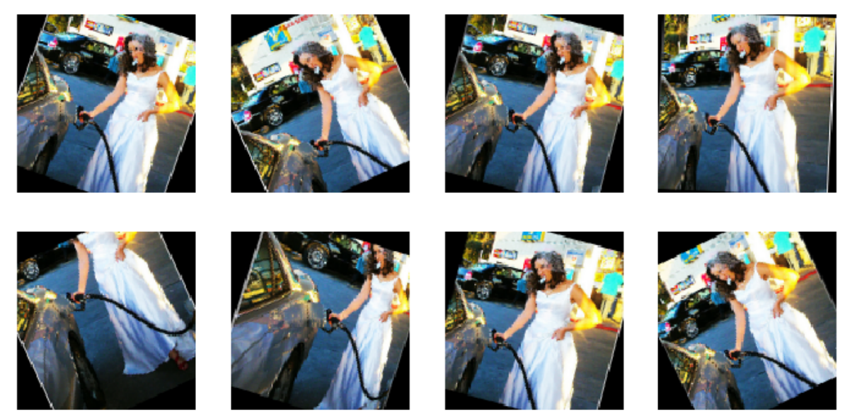
We can add a transform to do this perspective warping automatically with the rand resize and crop:
Question: How do you handle tabular, text, time series etc?
Text - read it. Time series - look at the signal. Tabular you would just visualize the augmented data the same way you would. All augmentations are domain specific. You need to know your data and domain well to invent your own augmentations. Make sure it makes sense and seems reasonable.
Question: What happens if the object of interest gets cropped out by image augmentation?
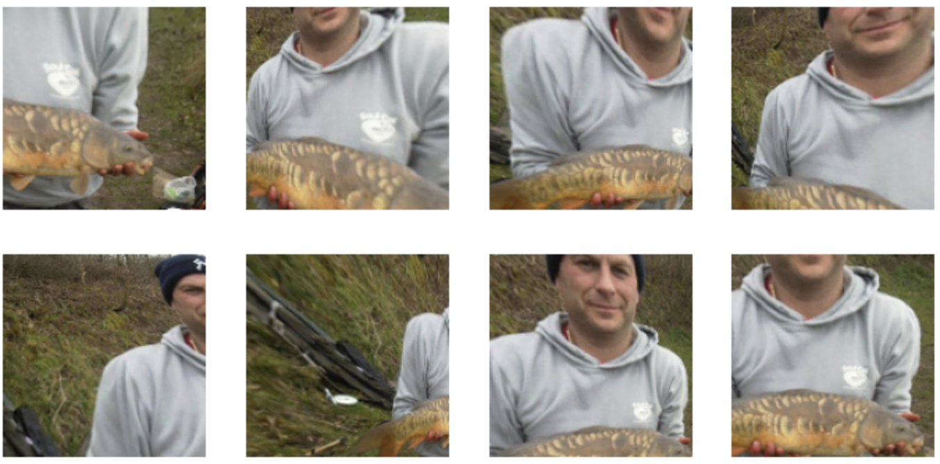
These are called noisy labels. Interesingly, the ImageNet winning stratedy with crop/zooming is to randomly pick 8-100% of the pixels. They very often have no tench. Or very often they have just the fin or just the eye. If we want to used crop/zooming well, we need to be very good at handling noisy labels (more in the next lesson). Also this tells you that if you already have noisy labels - don’t worry about it. All of the research we have tells us that we can handle noisy labels as long as it’s not biased.
It will also learn to recognize all the things associated with a tench. So if there’s a middle aged many outside looking happy - it could well be a tench! :)
Batch Data Augmentation
It’s actually possible to arbitrary affine transformation of images (rotating, zooming, shifting, warping etc) on the GPU. PyTorch provides all the functionality to make this happen. All the transformations need to happen after we create a batch. The key is to do them on a whole batch at a time. Nearly all PyTorch operations can be done batch-wise.
To do this we create a mini-batch of random numbers to create a mini-batch of augmented images.
An affine transform is basically a linear transform plus a translation. They are represented by matrices and multiple affine transforms can be composed by multiplying all their matrices together. (See this Blog post.)
Let’s load an image. Its shape is torch.Size([1, 3, 128, 128]).
Once we have resized our images so that we can batch them together, we can apply more data augmentation on a batch level. For the affine/coord transforms, we proceed like this:
1. Generate the Grid
A matrix is simply a function that takes a coordinate $(x, y)$ and maps them to some new location $(x’, y’)$. If we want to apply the same transformation to every pixel in an image, we first need to represent every pixel as a x,y coordinate.
Generate a grid map, using torch’s affine_grid, of the size of our batch (bs x height x width x 2) that contains the coordinates (-1 to 1) of a grid of size height x width (this will be the final size of the image, and doesn’t have to be the same as the current size in the batch).
def affine_grid(x, size):
    size = (size,size) if isinstance(size, int) else tuple(size)
    size = (x.size(0),x.size(1)) + size
    m = tensor([[1., 0., 0.], [0., 1., 0.]], device=x.device)
    return F.affine_grid(m.expand(x.size(0), 2, 3), size, align_corners=True)


grid = affine_grid(x, 128)
This has shape: torch.Size([1, 128, 128, 2]), and looks like:
tensor([[[[-1.0000, -1.0000],
          [-0.9843, -1.0000],
          [-0.9685, -1.0000],
          ...,
          [ 0.9685, -1.0000],
          [ 0.9843, -1.0000],
          [ 1.0000, -1.0000]],
				  ...,
         [[-1.0000,  1.0000],
          [-0.9843,  1.0000],
          [-0.9685,  1.0000],
          ...,
          [ 0.9685,  1.0000],
          [ 0.9843,  1.0000],
          [ 1.0000,  1.0000]]]])
Step 2: Affine Multiplication
Apply the affine transforms (which is a matrix multiplication) and the coord transforms to that grid map.
In 2D an affine transformation has the form y = Ax + b where A is a 2x2 matrix and b a vector with 2 coordinates. It’s usually represented by the 3x3 matrix
A[0,0]  A[0,1]  b[0]
A[1,0]  A[1,1]  b[1]
   0       0     1
because then the composition of two affine transforms can be computed with the matrix product of their 3x3 representations.
The matrix for a anti-clockwise rotation that has an angle of theta is:
cos(theta)  sin(theta) 0
-sin(theta) cos(theta) 0
0           0          1
then we draw a different theta for each version of the image in the batch to return a batch of rotation matrices (size bsx3x3).
You then multiply all 3 channels by the rotation matrix and add the translation:
tfm_grid = (torch.bmm(grid.view(1, -1, 2), m[:, :2, :2]) + m[:,2,:2][:,None]).view(-1, 128, 128, 2)
Step 3: Interpolate
Interpolate the values of the final pixels we want from the initial images in the batch, according to the transformed grid map using Pytorch’s F.grid_sample function:
def rotate_batch(x, size, degrees):
    grid = affine_grid(x, size)
    thetas = x.new(x.size(0)).uniform_(-degrees,degrees)
    m = rotation_matrix(thetas)
    tfm_grid = (torch.bmm(grid.view(1, -1, 2), m[:, :2, :2])  + m[:,2,:2][:,None]).view(-1, 128, 128, 2)
    return F.grid_sample(x, tfm_grid, align_corners=True)
Here is also a faster version using F.affine_grid:
def rotate_batch(x, size, degrees):
    size = (size,size) if isinstance(size, int) else tuple(size)
    size = (x.size(0),x.size(1)) + size
    thetas = x.new(x.size(0)).uniform_(-degrees,degrees)
    m = rotation_matrix(thetas)
    grid = F.affine_grid(m[:,:2], size)
    return F.grid_sample(x.cuda(), grid, align_corners=True)
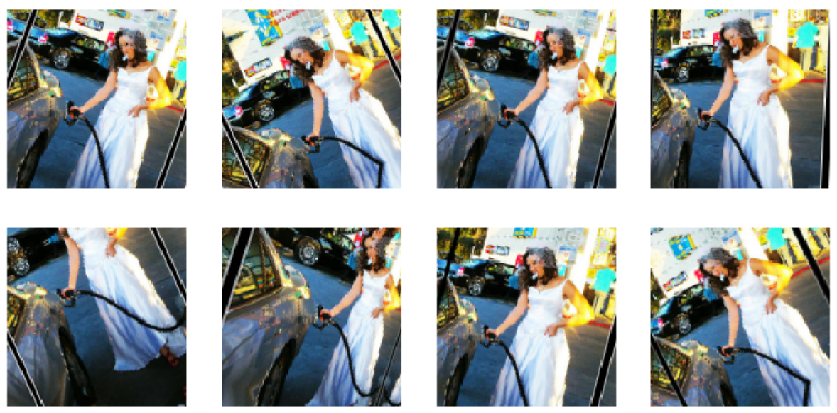
Results of this with random cropping and warping:
We get these black borders around the image. But PyTorch grid_sample also has a padding_mode argument that lets you filling in this black space in different ways - "zeros", "border", or "reflection". These can enrich and improve our augmented data even more. Here is reflection:
Links and References
-
Notebooks:
-
Papers:
- LSUV Paper: All You Need is a Good Init
- L2 Regularization versus Batch and Weight Normalization [2017]
- Three mechanisms of weight decay regularization [2019]
- Norm matters: Efficient and accurate normalization schemes in deep networks [2018]
- Jane Street Tech Blog - L2 Regularization and Batch Norm [2019]
- Adam Paper - Adam: A method for stochastic optimization [2015]
- Nesterov’s accelerated gradient and momentum as approximations to regularised update descent [2017]
- LAMB Paper - Large Batch Optimization for Deep Learning: Training BERT in 76 minutes [2019]
- LARS Paper - Large Batch Training of Convolutional Networks [2017] (LARS also uses weight statistics, not just gradient statistics.)
- Adafactor: Adaptive Learning Rates with Sublinear Memory Cost [2018] (Adafactor combines stats over multiple sets of axes)
- Adaptive Gradient Methods with Dynamic Bound of Learning Rate [2019]