Overview
This lesson covers a lot of material. It starts off with a review of some important foundations such as more advanced Python programming, variance, covariance, and standard deviation. It then goes into a short discussion on situation where Softmax loss is a bad idea in image classification tasks. My notes go deeper into this part on Multilabel classification than the original lecture does. The lesson then moves onto looking inside the model using PyTorch hooks. The last part of the lesson introduces Batch Normalization and studies the pros and cons of BatchNorm and shows some alternatives normalizations that are possible. Jeremy then develops a novel kind of normalization layer to overcome BatchNorm’s main problem, and compares it to previously published approaches, with some very encouraging results.
Lesson 10 lesson video.
Foundations
Notebook: 05a_foundations.ipynb
Mean: m = t.mean()
Variance: The average of how far away each data point is from the mean. Mean squared difference from the mean. Sensitive to outliers.
var = (t-m).pow(2).mean()- Better:
var = (t*t).mean() - (m*m) - $\mbox{E}[X^2] - \mbox{E}[X]^2$
Standard Deviation: Square root of the variance.
-
On same scale as the original data - easier to interpret.
-
std = var.sqrt()
Mean Absolute Deviation: Mean absolute difference from the mean. It isn’t used nearly as much as it deserves to be. Less sensitive to outliers than variance.
(t-m).abs().mean()
Covariance: A measure of how changes in one variable are associated with changes in a second variable. How linearly associated are two variables?
cov = ((t - t.mean()) * (v - v.mean())).mean()- $\operatorname{cov}(X,Y) = \operatorname{E}{\big[(X - \operatorname{E}[X])(Y - \operatorname{E}[Y])\big]} = \operatorname{E}[XY] - \operatorname{E}[X]\operatorname{E}[Y]$
cov = (t*v).mean() - t.mean()*v.mean()
Correlation: The strength and direction of the linear relationship between two variables.
- Covariance divided by the standard deviations of X and Y.
- $\rho_{X,Y}= \frac{\operatorname{cov}(X,Y)}{\sigma_X \sigma_Y}$
cor = cov / (t.std() * v.std())
See this: 3 minute video on Correlation vs Covariance.
MultiLabel Classification (When Softmax is a Bad Idea)
A common mistake many people make is using a Softmax where it isn’t appropriate. Recall the Softmax formula:
\[p(z_i) = \hbox{softmax(z)}_{i} = \frac{e^{z_{i}}}{\sum_{0 \leq j \leq n-1} e^{z_{j}}}\]In the Excel screenshot below, two different network outputs can produce the same Softmax output. This is weird, how does it happen?
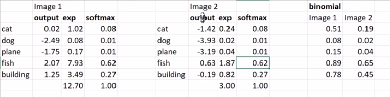
The sums of the exponentials for the two images (12.70 and 3.00) are dividing each of the exponentials and it happens that they come out with the exact same proportions for each category for both images.
In Image 1 there is a large activation for category “fish” (2.07), but in image 2 the activation for “fish” is only 0.63. Image 1 likely contains a fish, but it’s possible that image 2 doesn’t contain any of the categories. Softmax has to pick something however so it takes the weak fish activation and makes it big. It’s also possible that image 1 contains a cat, fish, and a building.
Put another way: many images are in fact multilabel, so Softmax is often a dumb idea, unless every one of your items has definitely at least one example of the thing you care about in it, and no items that have multiple examples in it. If an image doesn’t even have cat, dog, plane, fish, or building in it, it still has to pick something! Even if it has more than just one of the categories in it, it will have to pick one of them.
(N.B multiclass means one valid label per image, while multilabel means multiple labels per image. I always confuse these. Read this for a refresher.)
What do you do if there could there could be no things, or there could be more than one of these things? Instead you use a binary function where the output for each category in is:
\[B(z_i) = \frac{e^{z_i}}{1+e^{z_i}}\]This treats every category independently. The network assigns each category with a probability between 0 and 1, corresponding to how likely it thinks the category is present in the input data. (Note: the binary function is AKA the sigmoid function or logistic function).
The output of a binary function with the same example would look like:
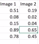
See how each category gets its own probability and is independent from all the others.
For image recognition, probably most of the time you don’t want Softmax. This habit comes from the fact that we all grew up with the luxury of ImageNet where the images are curated so that there is only one of each class in the image.
What if you instead added an additional category like “null”, “doesn’t exist”, “background”? This has been tried by researchers, but they found that it doesn’t work. The reason it doesn’t work is that we’d have to look for some set of features that correspond to “not cat/dog/plane/fish/building”. However this class of all things that are not something isn’t a kind of object so there isn’t some vector that can represent this.
Creating a binary has/has-not for each class is much easier for the network to learn. According to Jeremy: lots of well regarded papers make this mistake, so look out for it. If you suspect something does this, try replicating it without Softmax and you may just get a better result.
Example where Softmax is a good idea: language modelling -> predict the next word. There can be only one word next.
MultiLabel Predictions
Now that we understand the concept, what would this look like in code and how would we modify the loss function with the binary output layer?
Let’s first reproduce what Jeremy did in the Excel sheet in Python:
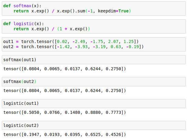
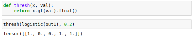
Where the logistic function is what Jeremy calls ‘binary’ in his lecture.
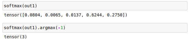
How do we interpret the outputs of softmax and logistic to get predictions? For Softmax layer the predicted label is the label with the highest output value. In code this is simply:
For the logistic output we need to threshold the values to filter in only the largest outputs. This threshold is user defined; 0.2 is used in fastai lesson 3 so let’s just go with that. Code:
MultiLabel Loss Function
What about the loss function for a logistic output? Recall from the last lesson that Softmax outputs a categorical probability distribution. With the numbers from the example above this is:
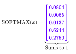
All the probabilities in a categorical distribution sum to 1 (I denote this property with the blue colour). Recall also from last lesson that the loss function used for a categorical distribution is the cross-entropy.
On the other hand, when we use the Binary/Logistic function the output isn’t a categorical distribution:
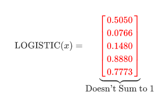
The probabilities in this vector don’t all sum to 1 (denoted with red) because they are all independent of each other. These probabilities are each the probability that the label is present in the data, independent of all the other labels. If we take 1 minus these probabilities we’d get the probability of the label not being present in the data. We can think of each of these as a 2-state system of present / not present and expand the vector out to include the not present probability:
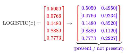
Now we can see that each of the rows is itself a categorical distribution with two categories (AKA Bernoulli distribution). Therefore to get the loss we can individually apply the cross-entropy loss to each of these distributions using target data (binary vector of present / not present for each label), then take the average of them all. You do that for every sample in the batch and then take the averages of all those averages to get the loss for the batch.
We don’t have to literally expand the vector out in practice, and can instead create a special case of the cross-entropy for this binary case, binary_cross_entropy:
def binary_cross_entropy(pred, targ):
    return -targ * pred.log() - (1 - targ) * (1 - pred).log()
The loss would be:
def multilabel_loss(out, targ):
    return binary_cross_entropy(logistic(out), targ).mean(1).mean(0)
Example use:
>>>out = torch.tensor([[0.02, -2.49, -1.75, 2.07, 1.25],
                       [-1.42, -3.93, -3.19, 0.63, -0.19]])
>>>targ = torch.tensor([[0., 0., 0., 1., 1.],
                        [1., 0., 0., 1., 1.]])

>>>multilabel_loss(out, targ)
tensor(0.4230)
This is a naive implementation of the loss, but it shows how it works. For a production implementation we need it to be more numerically stable (as discussed in last lesson) and do it all in log-space. We put the logistic function in log-space and then simplify things by fusing that with binary_cross_entropy. You can derive that the binary cross entropy with logistic function simplifies to:
Careful with the $e^x$, however, because it will overflow when $x$ isn’t even that large. To make things more numerically stable we employ the logsumexp trick again:
\[l(x, y) = m - yx + \log(e^{-m} + e^{x - m})\]Where $m = \max(x, 0)$. As code, this is:
def binary_cross_entropy_with_logits(out, targ):
    max_val = out.clamp_min(0.)
    return max_val - out * targ + ((-max_val).exp() + (out - max_val).exp()).log()
The loss function is modified to:
def multilabel_loss(out, targ):
    return binary_cross_entropy_with_logits(out, targ).mean(1).mean(0)
We’ve now recreated the loss function BCEWithLogitsLoss from PyTorch, which we can now use. Test with same example:
>>>out = torch.tensor([[0.02, -2.49, -1.75, 2.07, 1.25],
                       [-1.42, -3.93, -3.19, 0.63, -0.19]])
>>>targ = torch.tensor([[0., 0., 0., 1., 1.],
                        [1., 0., 0., 1., 1.]])

>>>loss = torch.nn.BCEWithLogitsLoss()
>>>loss(out, targ)
tensor(0.4230)
(Implementation in PyTorch (C++): binary_cross_entropy_with_logits)
Build a Learning Rate Finder
Notebook: 05b_early_stopping.ipynb, Jump to lesson 10 video
Better Callback Cancellation
In the last implementation of the Callback and Runner classes, stopping the training prematurely (e.g. for early stopping) was handled by callbacks returning booleans or by a attribute called stop getting set and checked at some point. This is a bit inflexible and also not very readable.
We can instead make use of Exceptions as a kind of control flow technique rather than just an error handling technique. You can subclass Exception to give it your own informative name without even changing its behaviour, like so:
class CancelTrainException(Exception): pass
class CancelEpochException(Exception): pass
class CancelBatchException(Exception): pass
Callbacks are free to raise Exceptions. The training loop can catch these and change control. This is a super neat and readable way that someone writing a callback can stop any of the three levels in the training loop from happening.
Refactoring Callback and Runner
Refactor/redesign the Callback and Runner class from last time. The Callback class now contains the ‘message passing’ (e.g. self('begin_fit') ) logic from before. This means that callback writers can now have control to override __call__ themselves in special cases, for debugging etc.
Here’s what the base class looks like now, alongside the default Training/Validation callback which holds the logic for the training or validating parts of the loop:
class Callback():
    _order, run = 0, None
    def set_runner(self, run):
        self.run=run
    def __getattr__(self, k):
        ## Get attributes from Runner object
        return getattr(self.run, k)

    @property
    def name(self):
        name = re.sub(r'Callback$', '', self.__class__.__name__)
        return camel2snake(name or 'callback')

    ## Refactored from before
    def __call__(self, cb_name):
        f = getattr(self, cb_name, None)
        if f and f(): return True
        return False

## DEFAULT Callback for Training/Validation
class TrainEvalCallback(Callback):
    def begin_fit(self):
        self.run.n_epochs=0.
        self.run.n_iter=0

    def after_batch(self):
        if not self.in_train: return
        self.run.n_epochs += 1./self.iters
        self.run.n_iter   += 1

    def begin_epoch(self):
        self.run.n_epochs=self.epoch
        self.model.train()
        self.run.in_train=True

    def begin_validate(self):
        self.model.eval()
        self.run.in_train=False
Notice how Callback and its subclasses can access attributes in Runner (set in the set_runner method) and even the getattr in Callback is overloaded to instead look in the Runner.
The __getattr__ overloading confused me for a while, until I realised how it actually works. Quote from this Stackoverflow question:
__getattr__is only called as a last resort i.e. if there are no attributes in the instance that match the name. For instance, if you accessfoo.bar, then__getattr__will only be called iffoohas no attribute calledbar. If the attribute is one you don’t want to handle, raiseAttributeError
Python looks for the attribute in the Callback first, if it can’t find it then it looks in the attributes of Runner.
This kind of strong coupling / encapsulation breaking made me a bit nervous initially, but after thinking about it more I think its a special design that works well in this unique setting. Runner and Callback are kind of like ‘friend classes’ from C++, where two friend classes ‘share’ their attributes with each other, but are still separate classes. By doing it this way, callback writers can gain privileged access to internals of the training loop, and so can inject code into the loop as if they were directly editing the source code of Runner.
Here is a skeleton of the code for Runner:
class Runner():
    def __init__(self, cbs=None, cb_funcs=None):
        cbs = listify(cbs)
        for cbf in listify(cb_funcs):
            cb = cbf()
            setattr(self, cb.name, cb)
            cbs.append(cb)
        self.cbs = [TrainEvalCallback()] + cbs

    @property
    def opt(self):       return self.learn.opt
    @property
    def model(self):     return self.learn.model
    @property
    def loss_func(self): return self.learn.loss_func
    @property
    def data(self):      return self.learn.data

    def one_batch(self, xb, yb):
        try:
			## INNER LOOP CODE
        except CancelBatchException: self('after_cancel_batch')
        finally: self('after_batch')

    def all_batches(self, dl):
        try:
            ## EPOCH CODE
        except CancelEpochException: self('after_cancel_epoch')

    def fit(self, epochs, learn):
        self.epochs, self.learn, self.loss = epochs, learn, tensor(0.)

        try:
            for cb in self.cbs: cb.set_runner(self)
            self('begin_fit')
            for epoch in range(epochs):
                self.epoch = epoch
                if not self('begin_epoch'):
					# TRAIN

                with torch.no_grad():
                    if not self('begin_validate'):
                        # VALIDATE
                self('after_epoch')

        except CancelTrainException: self('after_cancel_train')
        finally:
            self('after_fit')
            self.learn = None

    def __call__(self, cb_name):
        res = False
        for cb in sorted(self.cbs, key=lambda x: x._order):
            res = cb(cb_name) or res
        return res
I removed all the business code from the snippet, to save space and also so it could be implemented as an exercise.
LR_Find Callback
The learning rate finder is the work horse from part 1 of the fastai course. Let’s look at how to implement it and code that up as a callback.
LR_Find Algorithm Outline:
- Define upper and lower bounds for the learning rate and a number of steps. Lower should be small like
1e-10and the upper should be very layer like1e+2. Numbers of steps should be something like 100. - Start training the network with a learning rate starting at the lower bound.
- After every batch update, exponentially increase the learning rate and record the loss.
- If the learning rate hits the upper bound, or the loss ‘explodes’ then stop the process.
- After the finder has finished, plot the loss versus learning rate so we can eyeball the best learning rate.
To exponentially increase the learning rate using the formula:
\[lr_i = lr_{min} \left(\frac{lr_{max}}{lr_{min}}\right)^{i/i_{max}}\]‘Exploding’ loss can be defined as some factor (e.g. 10) times the lowest loss value recorded.
The code for the LR_Find callback is:
class LR_Find(Callback):
    _order=1
    def __init__(self, max_iter=100, min_lr=1e-6, max_lr=1):
        self.max_iter, self.min_lr, self.max_lr = max_iter, min_lr, max_lr
        self.best_loss = 1e9

    def begin_batch(self):
        if not self.in_train: return
        pos = self.n_iter / self.max_iter
        lr = self.min_lr * (self.max_lr / self.min_lr) ** pos
        for pg in self.opt.param_groups:
            pg['lr'] = lr

    def after_step(self):
        if self.n_iter >= self.max_iter or self.loss > self.best_loss*10:
            raise CancelTrainException()
        if self.loss < self.best_loss:
            self.best_loss = self.loss
Plot of loss versus learning rate:
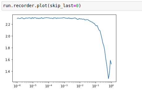
This PyImageSearch blog post is an excellent resource for learning more about LR Find and also uses exponential smoothing in the loss recordings too.
Build a CNN (with Cuda!)
Notebook: 06_cuda_cnn_hooks_init.ipynb, Jump to lesson 10 video
Let’s build a CNN for doing the MNIST problem using PyTorch and CUDA. Our simple CNN is a sequential model that contains a bunch of stride-2 convolutions, an average pooling, flatten, then a linear layer.
def get_cnn_model(data):
    return nn.Sequential(
        Lambda(mnist_resize),
        #         ni,nf,ksize
        nn.Conv2d( 1, 8, 5, padding=2,stride=2), nn.ReLU(), # 8x14x14
        nn.Conv2d( 8,16, 3, padding=1,stride=2), nn.ReLU(), # 16x7x7
        nn.Conv2d(16,32, 3, padding=1,stride=2), nn.ReLU(), # 32x4x4
        nn.Conv2d(32,32, 3, padding=1,stride=2), nn.ReLU(), # 32x2x2
        nn.AdaptiveAvgPool2d(1),    # 32x1
        Lambda(flatten),            # 32
        nn.Linear(32,data.c)        # 10
    )
The dimensions of the data as it flows through the model are provided in the comments. AdaptiveAvgPooling downsamples the data using an average.
Original data is vectors of 784 so they need to be reshaped to 28x28 to go into the convolution layers. We need to write a function mnist_resize to do this:
def mnist_resize(x):
    # batchsize, num_channels, height, width
    return x.view(-1, 1, 28, 28)
In order to turn helper functions into ‘layers’ that we can pass into nn.Sequential, we can create simple wrapper layer class Lambda(nn.Module) that takes this function and calls it in its forward method. This is used in the code above for calling mnist_resize and flatten.
Training this for one epoch on my laptop CPU took 7.14 seconds.
We need to speed this up using the GPU! To get started we need to prepare PyTorch to use the GPU. First check that Cuda is available to use with torch.cuda.is_available(), which should return True. Then set the device in PyTorch:
device = torch.device('cuda', 0)	# NB assumes only 1 GPU
torch.cuda.set_device(device)
To run on the GPU we need to do two things:
- Put the model on the GPU, i.e. the model’s parameters.
- Put the inputs and the loss function on the GPU, i.e. the things that come out of the dataloaders.
We can implement this with a callback:
class CudaCallback(Callback):
    def begin_fit(self):
        self.model.cuda()
    def begin_batch(self):
        self.run.xb, self.run.yb = self.xb.cuda(), self.yb.cuda()
At the beginning of the fit, put the model on the GPU. Before each batch starts, put the batch data on the GPU.
Adding this in training for 3 epochs took 7.12 s on my laptop - a nice 3x speedup. :)
Some Refactoring
First we can regroup all the conv/ReLU in a single function because they are always called together.
Next to refactor is the batch resizing for MNIST. This is hardcoded in the model, but we need something more general that could be used on other datasets. Of course this can be implemented as a callback! Make a callback BatchTransformXCallback for doing ‘transformations’ to the data before it goes into the model. Resize is one such possible transformation.
class BatchTransformXCallback(Callback):
    _order = 2
    def __init__(self, tfm):
        self.tfm = tfm # stores a transform
    def begin_batch(self):
        self.run.xb = self.tfm(self.xb) # transform the batch
So we have a resize or view transform to perform for each batch:
def view_tfm(*size):
    def _inner(x): return x.view(*((-1,)+size))
    return _inner

mnist_view = view_tfm(1,28,28)
cbfs.append(partial(BatchTransformXCallback, mnist_view))
Discussion on CNN Kernel Sizes
First conv layer on imagenet networks typically have 7x7 or 5x5 size kernels, while the rest of the conv layers use 3x3 kernels. Why is that?
If we just focus on MNIST, the first layer of the MNIST-CNN we only have a single channel image. We need to be mindful of what’s going on when we apply a kernel to this. If we have 8 3x3 filters then for a single point in the image we are converting 9 pixels (from 3x3 kernel) into a vector of 8 numbers (from 8 filters). We aren’t gaining anything from that, it’s basically shuffling the numbers around. For the first conv layer when we just have 1 or 3 channels people use a larger kernel size such as 7x7 or 5x5 in order to capture more information.
- 8 3x3 filters 1 channel => 9 -> 8
- 8 3x3 filters 3 channels => 27 -> 8
- 8 5x5 filters 1 channel => 25 -> 8
- 8 5x5 filters 3 channels => 75 -> 8
- 8 7x7 filters 1 channel => 49 -> 8
- 8 7X7 filters 3 channels => 147 -> 8
Later conv layers have more ‘channels’ so that isn’t an issue anymore. The deeper layers are typically 3x3.
Here are some useful discussions on this part of the lecture that helped me grok what Jeremy meant here: fastai forum, twitter.
Looking Inside the Model
We want to look inside of the model while it is training and see how the parameters are changing over time. Are they behaving themselves? Are they actually learning anything? Are there vanishing or exploding gradients?
PyTorch Hooks
Hooks are PyTorch’s version of callbacks, which are called inside of the model, and can be added, or registered, to any nn.Module. Hooks allow you to inject a function into the model that that is executed in either the forward pass (forward hook) or backward pass (backward hook). With hooks you can inspect / modify the output and grad of a layer. The hook can be a forward hook or a backward book.
A hook is attached to a layer, and needs to have a function that takes three arguments: module, input, output. Here we store the mean and std of the output in the correct position of our list.
class Hook():
    def __init__(self, m, f):
        self.hook = m.register_forward_hook(partial(f, self))
    def remove(self):
        self.hook.remove()
    def __del__(self):
        self.remove()


def append_stats(hook, mod, inp, outp):
    if not hasattr(hook,'stats'): hook.stats = ([],[],[])
    means,stds,hists = hook.stats
    means.append(outp.data.mean().cpu())
    stds .append(outp.data.std().cpu())
    hists.append(outp.data.cpu().histc(40,0,10)) #histc isn't implemented on the GPU
It’s very important to remove the hooks when they are deleted, otherwise there will be references kept and the memory won’t be properly released when your model is deleted.
Hooks class that contains several hooks:
class Hooks(ListContainer):
    def __init__(self, ms, f): super().__init__([Hook(m, f) for m in ms])
    def __enter__(self, *args): return self
    def __exit__ (self, *args): self.remove()
    def __del__(self): self.remove()

    def __delitem__(self, i):
        self[i].remove()
        super().__delitem__(i)

    def remove(self):
        for h in self: h.remove()
Having given an __enter__ and __exit__ method to our Hooks class, we can use it as a context manager. This makes sure that onces we are out of the with block, all the hooks have been removed and aren’t there to pollute our memory.
Current State of Affairs
Use the append_stats hook to look at the mean and std of the parameters in each of the layers.
The layer means:
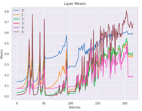
This looks awful. At the beginning of the training the values increase exponentially and then suddenly crash, repeatedly. It’s not training anything when this is happening. Eventually they settle down into some range and start to train. However are we sure that all the parameters are getting back to reasonable places after these ‘crashes’? Maybe the vast majority of them have zero gradients or are zero. Likely that this awful behaviour at the start of training is leaving the model in a really sad state.
The layer standard deviations:
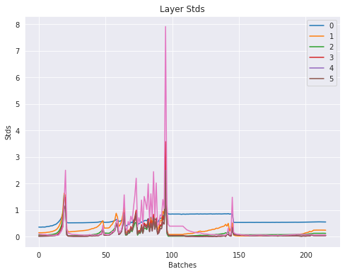
Subsequent layers standard deviations get closer and closer to 0. Later layers are basically getting 0 gradient.
Better Initialization
Use Kaiming init:
for l in model:
    if isinstance(l, nn.Sequential):
        init.kaiming_normal_(l[0].weight)
        l[0].bias.data.zero_()
Here are the layer means and stds now:
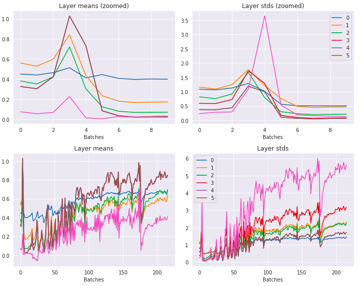
This is looking a lot better. No longer has the repeated exponential-crash pattern anymore. The standard deviations are all much closer to 1.
However these values are just aggregates of the layer parameters, so they don’t give us the full picture about how all the parameters are behaving. Rather than look at a single number we’d like to look at the distribution. To do that we can look at how the histogram of the parameters changes over time.
Here is a histogram of the activations, binned between 0 (relu) and 10 with 40 bins:
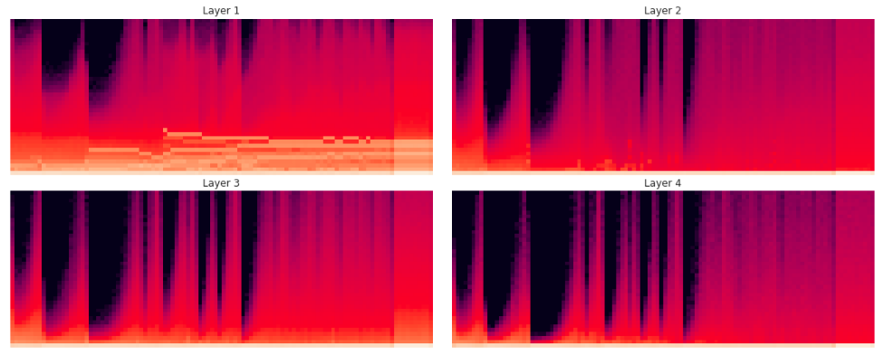
What we find is that even with Kaiming init, with the high learning rate we still get the same exponential-crash behaviour. The biggest concern is the amount of mass at the bottom of the histogram at 0.
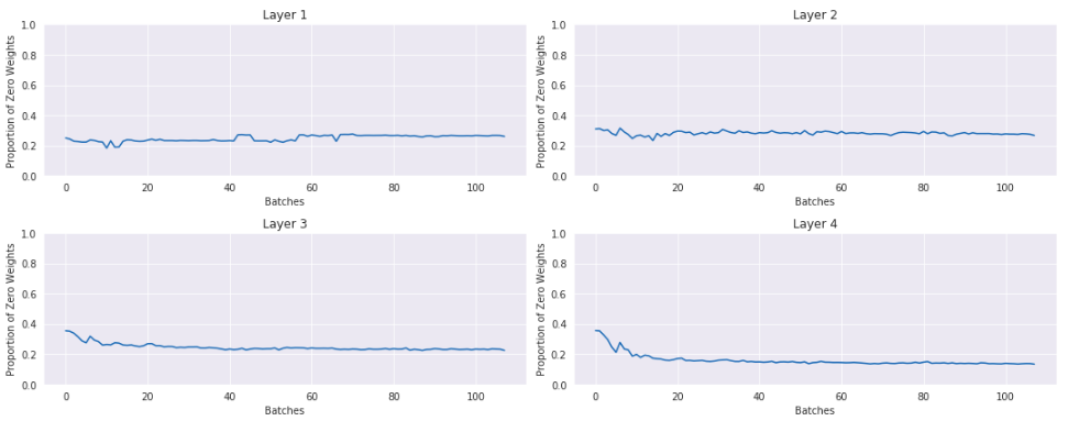
Here is a plot of the percentage of activations that are 0 or nearly 0:
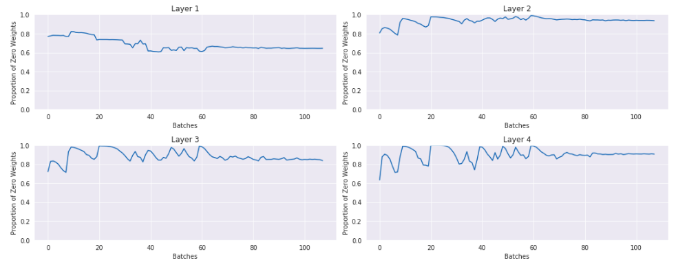
This is not good. In the last layer nearly 90% of the activations are actually 0. If you were training your model like this, it could appear like it was learning something, but you could be leaving a lot of performance on the table by wasting 90% of your activations.
Generalized ReLU
Let’s try to fix this so we can train a nice high learning rate and not have this happen. The main thing we will use to fix this is a GeneralRelu layer, where you can specify:
- An amount to subtract from the ReLU. (In earlier lesson it seemed that subtracting 0.5 from the ReLU might be a good idea.)
- Use leaky ReLU.
- Also the option of a maximum value.
Code for that:
class GeneralRelu(nn.Module):
    def __init__(self, leak=None, sub=None, maxv=None):
        super().__init__()
        self.leak,self.sub,self.maxv = leak,sub,maxv

    def forward(self, x):
        x = F.leaky_relu(x,self.leak) if self.leak is not None else F.relu(x)
        if self.sub is not None: x.sub_(self.sub)
        if self.maxv is not None: x.clamp_max_(self.maxv)
        return x
Retrain just like before with Kaiming init, and a GeneralRelu with parameters:
leak=0.1sub=0.4maxv=6.0
The layer means and standard deviations over time:
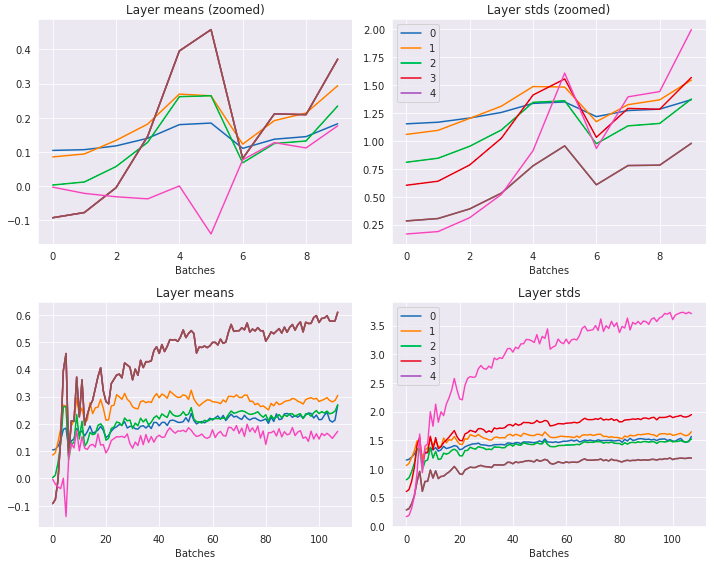
Looking better than before - means are around 0 and the stds are around 1 and are also a lot smoother looking.
Plot the histogram of the activations again, this time from -7 to 7 (leaky relu):
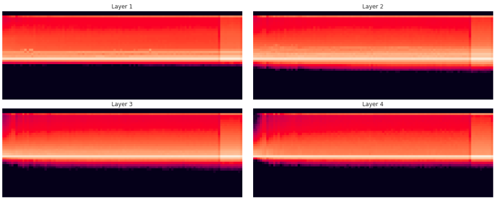
This is way better! It’s using the full richness of the possible activations. There’s not crashing of values.
How many of the activations are at or around zero:
The majority of the activations are not zero.
If we are careful about initialization, the ReLU, use one-cycle training, and a nice high learning rate of 0.9 we can achieve 98%-99% validation set accuracy after 8 epochs.
Normalization
Notebook: 07_batchnorm.ipynb
Batch Norm
Up to this point we have learned how to initialize the values to get better results. To get even better results we need to use normalization. The most common form of normalization is Batch Normalization. This was covered in Lesson 6, but here we implement it from scratch.
Algorithm from the BatchNorm paper:
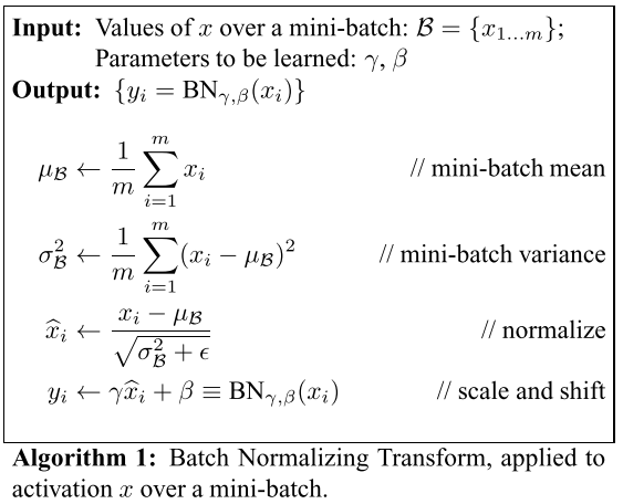
It normalizes the batch and scales and shifts it by $\gamma$ and $\beta$, which are learnable parameters in the model.
Here is that as code:
class BatchNorm(nn.Module):
    def __init__(self, nf, mom=0.1, eps=1e-5):
        super().__init__()
        # NB: pytorch bn mom is opposite of what you'd expect
        self.mom, self.eps = mom, eps
        self.mults = nn.Parameter(torch.ones (nf,1,1))
        self.adds  = nn.Parameter(torch.zeros(nf,1,1))
        self.register_buffer('vars',  torch.ones(1,nf,1,1))
        self.register_buffer('means', torch.zeros(1,nf,1,1))

    def update_stats(self, x):
        # x has dims (nb, nf, h, w)
        m = x.mean((0,2,3), keepdim=True)
        v = x.var ((0,2,3), keepdim=True)
        self.means.lerp_(m, self.mom)
        self.vars.lerp_ (v, self.mom)
        return m,v

    def forward(self, x):
        if self.training:
            with torch.no_grad(): m,v = self.update_stats(x)
        else: m,v = self.means,self.vars
        x = (x-m) / (v+self.eps).sqrt()
        return x*self.mults + self.adds
Let’s understand what this code is doing:
-
Instead of $\gamma$ and $\beta$, use descriptive names -
multsandadds. There is amultand anaddfor each filter coming into the BatchNorm. These are initialized to 1 and 0, respectively. -
At training time, it normalizes the batch data using the mean and variance of the batch. The mean calculation is:
x.mean((0,2,3), ...). The dimensions ofxare(nb, nf, h, w). So(0,2,3)tells it to take the mean over the batches, heights and widths, leavingnfnumbers. Same thing with the variance. -
However, at inference time every batch needs to be normalized with the same means and variances. If we didn’t do this, then if we get a totally different kind of image then it would remove all the things that are interesting about it.
-
While we are training, we keep an exponentially weighted moving average of the means and variances. The
lerp_method updates the moving average. These averages are what are used at inference time. -
These averages are stored in special way using:
self.register_buffer. This comes fromnn.Module. It works the same as a normal PyTorch tensor, except it moves the values to the GPU when the model is moved there. Also, we need to store these values the same way we store other parameters. This will save the numbers when the model is saved. We need to do this when we have ‘helper variables’ in a layer that aren’t parameters of the model. -
Another thing to note: if you use BatchNorm then the layer before doesn’t need to have a bias because BatchNorm has a bias already.
Exponentially Weighted Moving Average (EWMA)
The EWMA is a moving average that gives most weighting to recent values and exponentially decaying weight to older values. It allows you to keep a running average that is robust to outliers and requires that we keep track of only one number. The formula is:
\[\mu_t = \alpha x_t + (1 - \alpha)\mu_{t-1}\]Where $\alpha$ is called the momentum, which represents the degree of weight decrease. A higher value discounts older observations faster.
In PyTorch, EWMA is called ‘linear interpolation’ and uses the function means.lerp_(m, mom). In PyTorch the momentum in both lerp and in PyTorch’s BatchNorm uses opposite convention from everyone else, so you have to subtract value from 1 before you pass it. The default momentum in our code is 0.1.
(6 minute video with more info on EWMA)
Results
Training on MNIST with CNN, Kaiming init, BatchNorm, 1 epoch:
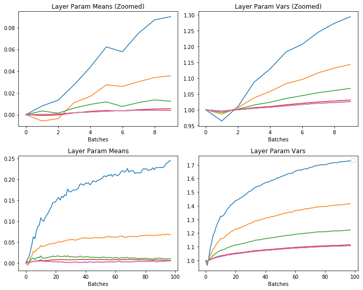
Working well. Means are all around 0 and the variances are all around 1.
BatchNorm Deficiencies
BatchNorm works great in most places, but it can’t be applied to online learning tasks, where we learn after every item. The problem is that the variance of one data point is infinite. You could also get the same problem if a single batch of any size contained all the same values. BatchNorm doesn’t work well for small batch sizes (like 2). This prohibits people from exploring higher-capacity models that would be limited by memory. It also can’t be used with RNNs.
tl;dr We can’t use BatchNorm with small batchsizes or with RNNs.
Layer Norm
LayerNorm is just like BatchNorm except instead of averaging over (0,2,3) we average over (1,2,3), and this doesn’t use the running average. Used in RNNs. It is not even nearly as good as BatchNorm, but for RNNs it is something we want to use because we can’t use BatchNorm.
From the LayerNorm paper: “batch normalization cannot be applied to online learning tasks or to extremely large distributed models where the minibatches have to be small”.
The difference with BatchNorm is:
- It doesn’t keep a moving average.
- It doesn’t average over the batches dimension, but over the hidden/channel dimension, so it’s independent of the batch size.
Code:
class LayerNorm(nn.Module):
    __constants__ = ['eps']
    def __init__(self, eps=1e-5):
        super().__init__()
        self.eps = eps
        self.mult = nn.Parameter(tensor(1.))
        self.add  = nn.Parameter(tensor(0.))

    def forward(self, x):
        m = x.mean((1,2,3), keepdim=True)
        v = x.var ((1,2,3), keepdim=True)
        x = (x-m) / ((v+self.eps).sqrt())
        return x*self.mult + self.add
Thought experiment: can this distinguish foggy days from sunny days (assuming you’re using it before the first conv)?
- Foggy days are less bright and have less contrast (lower variance).
- LayerNorm would normalize the foggy and sunny days to have the same mean and variance.
- Answer: no you couldn’t.
Instance Norm
The problem with LayerNorm is that it combines all channels into one. Instance Norm is a better version of LayerNorm where channels aren’t combined together. The key difference between instance and batch normalization is that the latter applies the normalization to a whole batch of images instead for single ones.
Code:
class InstanceNorm(nn.Module):
    __constants__ = ['eps']
    def __init__(self, nf, eps=1e-0):
        super().__init__()
        self.eps = eps
        self.mults = nn.Parameter(torch.ones (nf,1,1))
        self.adds  = nn.Parameter(torch.zeros(nf,1,1))

    def forward(self, x):
        m = x.mean((2,3), keepdim=True)
        v = x.var ((2,3), keepdim=True)
        res = (x-m) / ((v+self.eps).sqrt())
        return res*self.mults + self.adds
Used for Style transfer, not for classification. It’s included here as another example of normalization. You need to understand what it is doing in available to understand is it something that might work.
Group Norm
The Group Norm paper proposes a layer that divides channels into groups and normalizes the features within each group. GroupNorm is independent of batch sizes and it does not exploit the batch dimension, like how BatchNorm does. GroupNorm stays stable over a wide range of batch sizes. GroupNorm is supposed to solve the problem of BatchNorm with small batches.
It gets close to BatchNorm performance for ‘normal’ batch sizes in image classification, and beats BatchNorm with smaller batch sizes. GroupNorm works very well in large memory tasks such as: object detection, segmentation, and high resolution images.
It isn’t implemented in the lecture, but PyTorch has it already:
GroupNorm(num_groups, num_channels, eps=1e-5, affine=True)

>>> input = torch.randn(20, 6, 10, 10)
>>> # Separate 6 channels into 3 groups
>>> m = nn.GroupNorm(3, 6)
>>> # Separate 6 channels into 6 groups (equivalent with InstanceNorm)
>>> m = nn.GroupNorm(6, 6)
>>> # Put all 6 channels into a single group (equivalent with LayerNorm)
>>> m = nn.GroupNorm(1, 6)
>>> # Activating the module
>>> output = m(input)
(See this blog post for more details. This blog post covers even more kinds of initialization.)
Summary of the Norms with One Picture
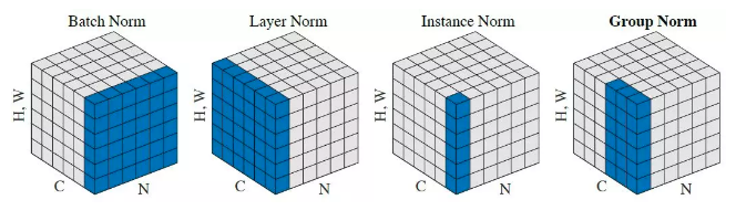
(Source)
In this diagram the height and width dimensions are flattened to 1D, so a single image is a ‘column’ in this diagram.
Running Batch Norm: Fixing Small Batch Size Problem
The normalizations above are attempts to work around the problem that you can’t use small batch sizes or RNNs with BatchNorm. But none of them are as good as BatchNorm.
Here Jeremy proposes a novel solution to solve the batch size problem, but not the RNN problem. This algorithm is called Running BatchNorm.
Algorithm idea:
- In the forward function, don’t divide by the batch standard deviation or subtract the batch mean, but instead use the moving average statistics at training time as well, not just at inference time.
- Why does this help? Let’s say you have batch size of 2. Then from time to time you may get a batch where the items are very similar and the variance is very close to 0. But that’s fine, because you are only taking 0.1 of that, and 0.9 of what you had before.
Code:
class RunningBatchNorm(nn.Module):
    def __init__(self, nf, mom=0.1, eps=1e-5):
        super().__init__()
        self.mom,self.eps = mom,eps
        self.mults = nn.Parameter(torch.ones (nf,1,1))
        self.adds = nn.Parameter(torch.zeros(nf,1,1))
        self.register_buffer('sums', torch.zeros(1,nf,1,1))
        self.register_buffer('sqrs', torch.zeros(1,nf,1,1))
        self.register_buffer('batch', tensor(0.))
        self.register_buffer('count', tensor(0.))
        self.register_buffer('step', tensor(0.))
        self.register_buffer('dbias', tensor(0.))

    def update_stats(self, x):
        bs,nc,*_ = x.shape
        self.sums.detach_()
        self.sqrs.detach_()
        dims = (0,2,3)
        s = x.sum(dims, keepdim=True)
        ss = (x*x).sum(dims, keepdim=True)
        c = self.count.new_tensor(x.numel()/nc)
        mom1 = 1 - (1-self.mom)/math.sqrt(bs-1)
        self.mom1 = self.dbias.new_tensor(mom1)
        self.sums.lerp_(s, self.mom1)
        self.sqrs.lerp_(ss, self.mom1)
        self.count.lerp_(c, self.mom1)
        self.dbias = self.dbias*(1-self.mom1) + self.mom1
        self.batch += bs
        self.step += 1

    def forward(self, x):
        if self.training: self.update_stats(x)
        sums = self.sums
        sqrs = self.sqrs
        c = self.count
        if self.step<100:
            sums = sums / self.dbias
            sqrs = sqrs / self.dbias
            c    = c    / self.dbias
        means = sums/c
        vars = (sqrs/c).sub_(means*means)
        if bool(self.batch < 20): vars.clamp_min_(0.01)
        x = (x-means).div_((vars.add_(self.eps)).sqrt())
        return x.mul_(self.mults).add_(self.adds)
Let’s work through this code.
- In normal BatchNorm we take the running average of the variance, but this doesn’t make sense - you can’t just average a bunch of variances. Particularly if the batch size isn’t constant. The way we want to calculate the variance is like this:
-
Let’s instead keep track of the sums
sumsand the sums of the squaressqrs, that store the EWMA of them. From the above formula - to get the means and variances we need to divide them by thecount(running average ofH*W*BS), which we also store as an EWMA. This accounts for the possibility of different batch sizes. -
We need to do something called Debiasing (aka bias correction). We want to make sure that no observation is weighted too highly. Normal way of doing EWMA gives the first point far too much weight. These first points are all zero, so the running averages are all biased low. Add a correction factor
dbias: $x_i = x_i/(1 - \alpha^i)$. When $i$ is large this correction factor tends to 1 - it only pushes up the initial values. (See this post). -
Lastly, to avoid the unlucky case of having a first mini-batch where the variance is close to zero, we clamp the variance to 0.01 for the first 20 batches.
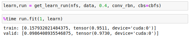
Results
With a batchsize of 2 and learning rate of 0.4, it totally nails it with just 1 epoch:
Links and References
- Lesson 10 lesson video.
-
Lesson 10 notebooks: 05a_foundations.ipynb, 05b_early_stopping.ipynb, 06_cuda_cnn_hooks_init.ipynb, 07_batchnorm.ipynb.
- Laniken Lesson 10 notes: https://medium.com/@lankinen/fast-ai-lesson-10-notes-part-2-v3-aa733216b70d
- Interpreting the colorful histograms used in this lesson
- Lecture on Bag-of-tricks for CNNs. Loads of state-of-the-art tricks for training CNNs for image problems, which would be a great exercise to reimplement as callbacks.
- Papers to read: