Overview
This lesson continues with the development of the MNIST model from the last lesson. It introduces and implements a Cross-entropy loss for MNIST, then takes a deep dive refactoring the model and the training loop, where it builds the equivalent classes from PyTorch from scratch, which provides a great foundation for understanding the main PyTorch classes. In the second half, the lesson moves onto the implementation of Callbacks and how they are integrated into the training loop in the FastAI library. Then it shows how to implement one-cycle training using the callback infrastructure that was built.
Lesson 9 lecture video.
I found the second half of this lesson hard to make notes for because it is so code heavy. I didn’t want to just reproduce the jupyter notebooks here. I instead opted to provide a companion to the notebooks, providing extra explanation and also motivation for the design decisions. I tried to write it such that they could be used as guide for implementing the main parts yourself from scratch, which is how I practice this course. Enjoy!
Classification Loss Function
From the last lesson the model so far is:
class Model(nn.Module):
    def __init__(self, n_in, nh, n_out):
        super().__init__()
        self.layers = [nn.Linear(n_in,nh), nn.ReLU(), nn.Linear(nh,n_out)]

    def __call__(self, x):
        for l in self.layers: x = l(x)
        return x
Recall we were using the MSE as the loss function, which doesn’t make sense for a multi-classification problem, but was convenient as a teaching tool. Let’s continue with this and use an appropriate loss function.
This follows the notebook: 03_minibatch_training.ipynb
Cross-Entropy Loss
We need a proper loss function for MNIST. This is a multi-class classification problem so we use Cross-entropy loss. Cross-entropy loss is calculated using a function called the Softmax function:
\[p(z_i) = \hbox{softmax(z)}_{i} = \frac{e^{z_{i}}}{\sum_{0 \leq j \leq n-1} e^{z_{j}}}\]Where $z_i$ are the real-valued outputs of the model. Softmax takes in a vector of $K$ real numbers, and normalizes it into a probability distribution of $K$ probabilities proportional to the exponentials of the input numbers. These collectively sum to 1, and each have values between 0 and 1 (this is also called a Categorical distribution).
We now have a probability vector (length 10), $p(z_i)$, that the model thinks that a given input has label $i$ (i.e. 0-9). This could look like:
pz = [0.05, 0.05, 0.05, 0.05, 0.1,
      0.6, 0.025, 0.025, 0.025, 0.025]
When training know what the target value is. If this is represented as a categorical distribution like $z$, we would get the vector $x$:
x = [0., 0., 0., 0., 0.,
     1.0, 0., 0., 0., 0.]
We know for certain what the target value is, so the probability for that label is 1 and the rest are 0. So we could think of this as a distribution, or just as a one-hot encoded vector for the target label.
Cross-entropy is a function commonly used to quantify the difference between two probability distributions, this is why we can use it as our loss function. If we have the ‘true’ distribution, $x_i$, and the estimated distribution, $p(z_i)$, the cross-entropy loss is defined as:
\[L =-\sum_i x_i \log p(z_i)\]This has a minimal value when the estimated distribution matches the true distribution. You can see this in the plot of the cross entropy with varying $p(z)$:
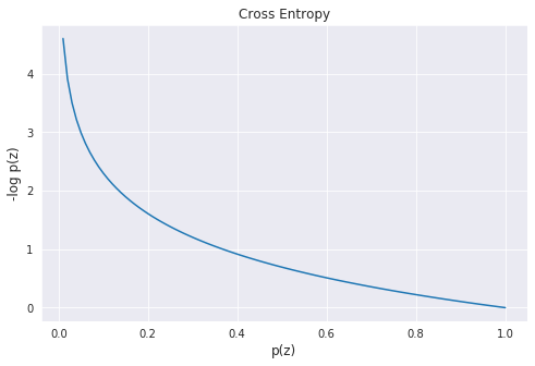
Another name for cross entropy is the negative log likelihood.
Since $x$ is a one-hot encoded vector, all the 0 entries will be masked out leaving the cross entropy as just:
\[L = -\log p(z_i) = -\log (\mbox{softmax}(\mathbf{z})_i)\]Where $i$ is the index of the target label. We can therefore code the cross-entropy loss for multi-class as an array lookup. The code for the cross-entropy, or negative log likelihood, is therefore:
def nll(input, target):
    # input is log(softmax(z))
    # x is 1-hot encoded target, so this simplifies to array lookup.
    return -input[range(target.shape[0]), target].mean()
The total loss is just the average of the negative log likelihood’s of all the training examples (in a batch). Next we need to implement a log-Softmax function to calculate the input to nll.
Log-Softmax Layer: Naive Implementation
First implementation: let’s code up the formula for Softmax then take the log of it:
def log_softmax(x):
    # naive implementation
	return (x.exp() / x.exp().sum(-1, keepdim=True)).log()
On paper, the maths works out and we can just convert the formula to code like above. However, this implementation has several big problems that mean this code will not work in practice.
Exponentials, Logs, and Floating Point Hell…
Working with exponentials on a computer requires care - these numbers can get very big or very small, fast. Floating point numbers are finite approximation of real numbers; for most of the time we can pretend that they behave like real numbers, but when we start to get into extreme values this thinking breaks down and we are confronted with the limitations of floats.
If a float gets too big it will overflow, that is it will go to INF:
np.exp(1) -> 2.718281828459045
np.exp(10) -> 22026.465794806718
np.exp(100) -> 2.6881171418161356e+43
np.exp(500) -> 1.4035922178528375e+217
np.exp(1000) -> inf # oops...
On the other hand, if a float gets too small it will underflow, that is it will go to zero:
np.exp(-1) -> 0.36787944117144233
np.exp(-10) -> 4.5399929762484854e-05
np.exp(-100) -> 3.720075976020836e-44
np.exp(-500) -> 7.124576406741286e-218
np.exp(-1000) -> 0.0 # oops...
The input to exponential doesn’t even have to that big to get under/overflow. Therefore we can’t really trust the naive softmax not to break because of this.
Another less obvious issue is that when doing operations on floats with extreme values, arithmetic can stop working:
np.exp(-10) + np.exp(-100) == np.exp(-10) # wut
np.exp(10) + np.exp(100) == np.exp(100) # wut?
Operations between floats are performed and then rounded. The difference in value between the numbers here is so massive that the smaller one gets rounded away and disappears - loss of precision. This is a big problem for the sum of exponentials in the denominator of the softmax formula.
The solution to dealing with extreme numbers is to transform everything into log space, where things are more stable. A lot of numerical code is implemented in log space and there are many formulae/tricks for transforming operations into log space. The easy ones are:
\[\begin{align} \log e^x &= x \\ \log b^a &= a \log b \\ \log (ab) &= \log a + \log b \\ \log \left ( \frac{a}{b} \right ) &= \log(a) - \log(b) \end{align}\]How to transform the sum of exponentials in softmax? There is no nice formula for the log of a sum, so we’d have to leave log space, compute the sum, and then take the log of it. Leaving log space would give us all the headaches described above. However there is trick to computing the log of a sum stably called the LogSumExp trick. The idea is to use the following formula:
\[\log \left ( \sum_{j=1}^{n} e^{x_{j}} \right ) = \log \left ( e^{m} \sum_{j=1}^{n} e^{x_{j}-m} \right ) = m + \log \left ( \sum_{j=1}^{n} e^{x_{j}-m} \right )\]Where $m$ is the maximum of the $x_{j}$. The subtraction of $m$ is to bring the numbers down to a size that’s safe to leave log land to perform the sum.
(Nerdy extras: even if a float isn’t so small that it underflows, if it gets small enough it becomes ‘denormalized’. Denormal numbers extend floats to get some extra values very close to zero. They are handled differently from normal floats by the CPU and their performance is terrible, slowing your code right down. See this classic stackoverflow question for more on this).
Log-Softmax Layer: Better Implementation
Implement LogSumExp in Python:
def logsumexp(x):
    m = x.max(dim=-1)[0]
    return m + (x - m.unsqueeze(-1)).exp().sum(dim=-1).log()
PyTorch already has this: x.logsumexp().
We can now implement log_softmax and cross_entropy_loss:
def log_softmax(x):
  # return x - x.logsumexp(-1,keepdim=True) # pytorch version
    return x - logsumexp(x).unsqueeze(-1)

def cross_entropy_loss(output):
    return nll(log_softmax(output), target)
Now we’ve implemented cross entropy from scratch we may use PyTorch’s versions of the functions:
import torch.nn.functional as F

test_near(F.nll_loss(F.log_softmax(pred, -1), y_train), loss)

test_near(F.cross_entropy(pred, y_train), loss)
Mini-Batch Training
Basic Training Loop
Now we have the loss function done, next we need a performance metric. For a classification problem we can use accuracy:
def accuracy(out, targ):
	return (torch.argmax(out, dim=1) == targ).float().mean()
Now we built a training loop. (Recall the training loop from Fast.ai part 1).
The basic training loop repeats over the following:
- Get the output of model on a batch of inputs
- Compare the output with the target and compute the loss
- Calculate the gradients of the loss wrt every parameter of the model
- Update the parameters using those gradients to make them a little bit better
In Python with our current model this is:
for epoch in range(epochs):
    for i in range((n-1)//bs + 1):
        start_i = i*bs
        end_i = start_i+bs
        xb = x_train[start_i:end_i]
        yb = y_train[start_i:end_i]
        loss = loss_func(model(xb), yb)

        loss.backward()
        with torch.no_grad():
            for l in model.layers:
                if hasattr(l, 'weight'):
                    l.weight -= l.weight.grad * lr
                    l.bias   -= l.bias.grad   * lr
                    l.weight.grad.zero_()
                    l.bias  .grad.zero_()
What it does:
loss.backward()computes the gradient of the loss wrt the parameters of the model using Pytorch’s autograd.- The updating of the parameters is done inside of
torch.no_grad()because this is not part of the gradient calculation, it’s the result of it. - It loops through the layers and checks if they have attribute ‘weight’.
- After updating the parameters it zeros the gradients so that the old values don’t persist into the next iteration.
The next part of the lesson works on refactoring this loop until we end up with an implementation equivalent to the one in PyTorch. I think it’s a good exercise to try and reproduce this yourself after watching this part of the lecture. Rather than just copy the notebook, I will structure this section as hints/descriptions of what you need to do, followed by the solution code from the notebook.
Refactoring 1
Currently when we update the parameters we have to loop through the layers and then check to see if they have parameter ‘weight’ and then update the weight and bias of that layer. This is long winded and it exposes the implementation too much.
We want instead to be able to loop through all the parameters in the model in a cleaner way:
...
            loss.backward()
            with torch.no_grad():
                for p in model.parameters():
                    p -= p.grad * lr
                model.zero_grad()
Hint: Our model already is a subclass of nn.Module, which has a special way of handling its attributes (__setattr__) that we can take advantage of if we change the way the layers are declared. Doing it this way will enable the use of nn.Module methods .parameters and .zero_grad…
Solution:
class Model(nn.Module):
    def __init__(self, n_in, nh, n_out):
        super().__init__()
        self.l1 = nn.Linear(n_in,nh)
        self.l2 = nn.ReLU()
        self.l3 = nn.Linear(nh,n_out)

    def __call__(self, x):
        return self.l3(self.l2(self.l1(x)))
Set the layers as attributes rather than storing a list of them. Doing things this way enables nn.Module to do some magic in the background. Look at the string representation of our model now:
>>> model
Model(
  (l1): Linear(in_features=784, out_features=50, bias=True)
  (l2): ReLU()
  (l3): Linear(in_features=50, out_features=10, bias=True)
)
It somehow knows about the layers we set as attributes. Looping through .parameters now returns the weight and bias matrices of the layers too.
What’s actually going on is nn.Module class overrides __setattr__, so every time we set an attribute that’s a PyTorch layer it registers that to an internal list. Methods like .parameters and .zero_grad then iterate through that list.
This internal list is stored as self._modules, we can take a peek at it:
>>> model._modules
OrderedDict([('l1', Linear(in_features=784, out_features=50, bias=True)),
             ('l2', ReLU()),
             ('l3', Linear(in_features=50, out_features=10, bias=True))])
Refactoring 2
It’s more convenient now, but it’s not convenient enough. It’s not nice having to write attributes for every layer - what if we had 50 layers? The forward pass is also inconvenient to write, it was better when we could just loop through the layers.
It would be nice if we could make the old implementation that had a list of layers work while getting the __setattr__ goodness too.
Hint: checkout nn.ModuleList
Solution:
class SequentialModel(nn.Module):
    def __init__(self, layers):
        super().__init__()
        self.layers = nn.ModuleList(layers)

    def __call__(self, x):
        for l in self.layers:
            x = l(x)
        return x
``nn.ModuleList` gives us the list model, but also registers the layers in the list so we retain the nice features from before:
>>> model
SequentialModel(
  (layers): ModuleList(
    (0): Linear(in_features=784, out_features=50, bias=True)
    (1): ReLU()
    (2): Linear(in_features=50, out_features=10, bias=True)
  )
)
We have implemented the equivalent to nn.Sequential, which we now may use.
model = nn.Sequential(nn.Linear(m, nh), nn.ReLU(), nn.Linear(nh, nout))
Checkout the source code for this and see how similar the code is to our version: nn.Sequential??.
Refactoring 3
That’s the model refactored. What about the optimization step? Let’s replace our previous manually coded optimization step:
with torch.no_grad():
    for p in model.parameters(): p -= p.grad * lr
    model.zero_grad()
and instead use just:
opt.step()
opt.zero_grad()
This abstracts away the optimization algorithm and implementation and lets us swap things out in future.
Hint: Let’s create a class Optimizer to do this. It should take the parameters and the learning rate and implement the step and zero_grad methods.
Solution:
class Optimizer():
    def __init__(self, params, lr=0.05):
        self.params = list(params)
        self.lr = lr

    def step(self):
        with torch.no_grad():
            for p in self.params:
                p -= p.grad * self.lr

    def zero_grad(self):
        for p in self.params:
            p.grad.zero_()
Training loop is now:
opt = Optimizer(model.parameters())

for epoch in range(epochs):
    for i in range((n-1)//bs + 1):
        start_i = i*bs
        end_i = start_i+bs
        xb = x_train[start_i:end_i]
        yb = y_train[start_i:end_i]
        pred = model(xb)
        loss = loss_func(pred, yb)

        loss.backward()
        opt.step()
        opt.zero_grad()
We now implemented an equivalent of PyTorch’s optim.SGD, which we may now use:
from torch import optim

opt = optim.SGD(model.parameters(), lr=0.05)
Refactoring 4 - Dataset
Let’s refactor how the data is retrieved and grouped into batches.
It’s clunky to iterate through minibatches of x and y values separately:
xb = x_train[start_i:end_i]
yb = y_train[start_i:end_i]
Instead, let’s do these two steps together, by introducing a Dataset class:
xb, yb = train_ds[i*bs : i*bs+bs]
Hint: your class needs to override __getitem__.
Solution:
class Dataset():
    def __init__(self, x, y):
        self.x, self.y = x, y
    def __len__(self):
        return len(x)
    def __getitem__(self):
        return self.x[i], self.y[i]
Use:
train_ds,valid_ds = Dataset(x_train, y_train),Dataset(x_valid, y_valid)
Refactoring 5 - DataLoader
Previously, our loop iterated over batches (xb, yb) like this:
for i in range((n-1)//bs + 1):
    xb,yb = train_ds[i*bs : i*bs+bs]
    ...
Let’s make our loop much cleaner, using a data loader:
for xb,yb in train_dl:
    ...
Hint: you need to override __iter__ and use yield.
Solution:
class DataLoader():
    def __init__(self, ds, bs):
        self.ds,self.bs = ds,bs
    def __iter__(self):
        for i in range(0, len(self.ds), self.bs):
            yield self.ds[i:i+self.bs]
Use, training and validation data loaders:
train_dl = DataLoader(train_ds, bs)
valid_dl = DataLoader(valid_ds, bs)
After all this refactoring the training loop now looks like:
def fit():
    for epoch in range(epochs):
        for xb,yb in train_dl:
            pred = model(xb)
            loss = loss_func(pred, yb)
            loss.backward()
            opt.step()
            opt.zero_grad()
Much smaller and very readable.
Random Sampling
We want our training set to be in a random order, and that order should differ each iteration. But the validation set shouldn’t be randomized.
As we did with DataLoader we can implement this as a class that takes a Dataset and batch size, then overrides _iter__ so that it yields the indices of the dataset in a random order.
class Sampler():
    def __init__(self, ds, bs, shuffle=False):
        self.n,self.bs,self.shuffle = len(ds),bs,shuffle

    def __iter__(self):
        self.idxs = torch.randperm(self.n) if self.shuffle else torch.arange(self.n)
        for i in range(0, self.n, self.bs):
            yield self.idxs[i:i+self.bs]
Use:
s = Sampler(small_ds,3,True)
[o for o in s]
We can then update our DataLoader class so that it takes a Sampler and can return items in a random order.
def collate(b):
    xs,ys = zip(*b)
    return torch.stack(xs),torch.stack(ys)

class DataLoader():
    def __init__(self, ds, sampler, collate_fn=collate):
        self.ds,self.sampler,self.collate_fn = ds,sampler,collate_fn

    def __iter__(self):
        for s in self.sampler:
            yield self.collate_fn([self.ds[i] for i in s])
The collate function is for gathering up the data in the batch. In this case [self.ds[i] for i in s] returns a list of (x,y) tuples. We want these to be instead be two tensors xs and ys, which is what the function collate does.
Use:
train_samp = Sampler(train_ds, bs, shuffle=True)
valid_samp = Sampler(valid_ds, bs, shuffle=False)

train_dl = DataLoader(train_ds, sampler=train_samp, collate_fn=collate)
valid_dl = DataLoader(valid_ds, sampler=valid_samp, collate_fn=collate)
End Product Implemented with PyTorch Classes
At this point we have implemented the equivalents of the PyTorch classes: DataLoader, SequentialSampler, and RandomSampler, so we may use them from now on.
The PyTorch code that does everything we have implemented so far would be:
from torch.utils.data import DataLoader
import torch.functional as F
from torch import optim


train_ds = Dataset(x_train, y_train)
valid_ds = Dataset(x_valid, y_valid)
train_dl = DataLoader(train_ds, bs, shuffle=True, drop_last=True)
valid_dl = DataLoader(valid_ds, bs, shuffle=False)

loss_func = F.cross_entropy


def get_model():
    model = nn.Sequential(nn.Linear(m, nh), nn.ReLU(), nn.Linear(nh, 10))
    opt = optim.SGD(model.parameters(), lr=0.05)
    return model, opt


def fit(epochs, model, loss_func, opt, train_dl, valid_dl):
    for epoch in range(epochs):
        # train
        model.train()
        for xb, yb in train_dl:
            loss = loss_func(model(xb), yb)
            loss.backward()
            opt.step()
            opt.zero_grad()

        # validate
        model.eval()
        with torch.no_grad():
            total_loss, total_acc = 0.0, 0.0
            for xb, yb in valid_dl:
                pred = model(xb)
                total_loss += loss_func(pred, yb)
                total_acc += accuracy(pred, yb)
        nv = len(valid_dl)
        # NB these averages are incorrect if the
        # batch size varies...
        print(epoch, total_loss/nv, total_acc/nv)

fit(3, model, loss_func, opt, train_dl, valid_dl)
This training loop also includes validation. We calculate and print the validation loss at the end of each epoch.
Note that we always call model.train() before training, and model.eval() before inference, because these are used by layers such as nn.BatchNorm2d and nn.Dropout to ensure appropriate behaviour for these different phases.
Infinitely Customizable Training Loop
Our train loop so far is in the function fit above. We need a code design where users can infinitely customize this loop to add whatever they want, like fancy progress bars, different optimizers, tensorboard integration, regularization etc. The library design would need to be open and flexible enough to handle any unforeseen extensions. There is a good way to build something that can handle this - Callbacks.
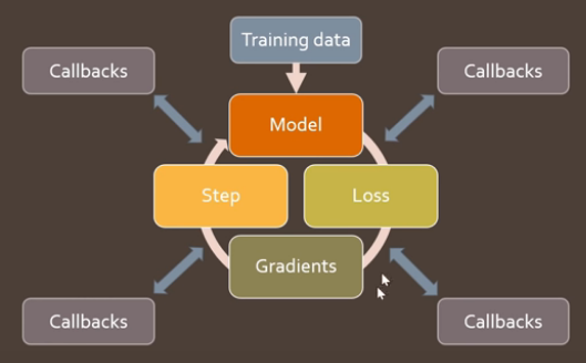
FastAI’s callbacks not only let you look at, but fully customize every single part of the training loop. The training loop contains all the parts of the code we wrote above, but in between these parts are slots for callbacks. Like on_epoch_begin, on_batch_begin, on_batch_end, on_loss_begin… and so on. Screen grab from lecture:
These updates can be new values, or flags that skip steps or stop the training.
With this we can create all kinds of useful stuff in FastAI like learning rate schedulers, early stopping, parallelism, or gradient clipping. You can also mix them all together.
This next part of the lesson builds the framework for handling callbacks. It’s hard to write as notes because it is very code heavy. I will make some general descriptions of the design decisions. Then I will move onto the implementations of Callbacks used within this framework. I recommend just watching the lesson and working through the notebook.
Training Loop Landmarks
The training loop has several key points or landmarks just before or just after important parts of the training loop and we may want to inject some functionality/code into those points. In running order these are:
- The start of the training:
begin_fit - The end of the training:
after_fit - The start of each epoch:
begin_epoch - The start of a batch:
begin_batch - After the loss is calculated:
after_loss - After the backward pass is performed:
after_backward - After the optimizer has performed a step:
after_step - After all the batches and before validation:
begin_validate - The end of each epoch:
after_epoch - The end of the training:
after_fit - Also after every batch or epoch we may want to halt everything:
do_stop
Callback Class + Callback Handler (Version 1)
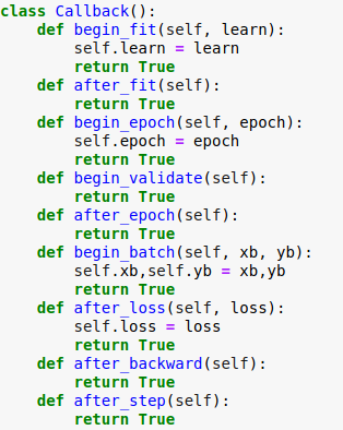
A sensible design option when faced with this would be to define an abstract base class that has methods corresponding to all the landmarks (+ method names) above. Every one of these methods should return True or False to indicate success/failure or some other stopping condition. At each of the landmarks in the training loop these booleans will be checked to see if the training loop should continue or not.
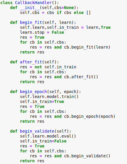
What the Callback base class could look like:
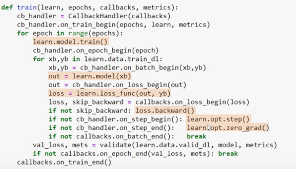
We want to be able to pass multiple callbacks to the training loop so we’d need an addition class to handle collections of callbacks called CallbackHandler. It would have a collection of Callback objects and the same methods as Callback except it loops through all of its callback objects and return a boolean indicated if all the callbacks were successful or if any failed.
Here is a snippet of a potential CallbackHandler class:
Alternative Design: Runner Class
The last design could lead to some code smell as seen here:
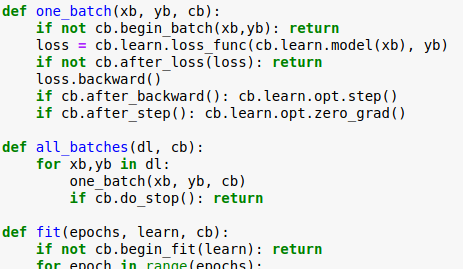
Callbacks cb are passed as the argument of every function in the training loop. This suggests that these functions should be part of a class and cb should be an instance attribute in that class.
We create a new class Runner (I won’t list here), which contains one_batch, all_batches, and fit methods from the training loop, takes a list of Callback objects in the constructor, while also integrating the logic of the the previous CallbackHandler class.
It has some clever refactoring so that the looping through the callbacks is handled by overriding __call__, finding all the callbacks in its collection that have the required method name (e.g. ‘begin_epoch’) and calling them. The boolean logic of starting and stopping is handled by this method too, which means the Callback subclasses no longer need to return booleans - they can just do their job without needing to know the context within which they are used. Here is an example of a Callback in this implementation:
class ChattyCallback(Callback):
    def begin_epoch(self):
        print('begin_epoch...')
    def after_epoch(self):
        print('after epoch...')
    def begin_fit(self):
        print('begin_fit...')
    def begin_validate(self):
        print('begin_validate...')
>>> run = Runner(cbs=[ChattyCallback()])
>>> run.fit(2, learn)
begin_fit...
begin_epoch...
begin_validate...
after epoch...
begin_epoch...
begin_validate...
after epoch...
The Runner design decouples the training loop from the callbacks such that even the different logic required for training and validation parts of the training loop can be implemented as a Callback which is hard coded into the Runner class:
class TrainEvalCallback(Callback):
    def begin_fit(self):
        self.run.n_epochs=0.
        self.run.n_iter=0

    def after_batch(self):
        if not self.in_train: return
        self.run.n_epochs += 1./self.iters
        self.run.n_iter   += 1

    def begin_epoch(self):
        self.run.n_epochs=self.epoch
        self.model.train()
        self.run.in_train=True

    def begin_validate(self):
        self.model.eval()
        self.run.in_train=False
(IMHO: The Runner code is quite hard to understand, but it’s not important in the rest of the course. This is an experimental class and it doesn’t end up even in the FastAI2 library. Looking at the state of the library (2/2020), ideas from this class do appear in the new Learner class. It’s better just to know what you need to write callbacks).
Things to note for all the Callbacks implemented in the next section:
- They assume the existence of
self.in_train, denoting if we are in training or validation. This variable is set byTrainEvalCallback. - They also have access to variables in the
Runnerclass such as:self.opt,self.model,self.loss_func,self.data,self.n_epochs, andself.epochs.
Callbacks Applied: Annealing
Rather than spend too much time on understanding Runner, let’s move onto doing something useful - implementing some callbacks.
Let’s implement callbacks to do one-cycle training. If you can train the first batches well, then the whole training will be better, and you can get super-convergence. Good annealing is critical to doing the first few batches well.
First let’s make a callback Recorder that records the learning rate and loss after every batch. This calls will need two lists for the learning rates and the losses that are initialized at the being of the training loop, and it will need to append to these lists after every batch.
Recorder:
class Recorder(Callback):
    def begin_fit(self): self.lrs,self.losses = [],[]

    def after_batch(self):
        if not self.in_train: return
        self.lrs.append(self.opt.param_groups[-1]['lr'])
        self.losses.append(self.loss.detach().cpu())

    # methods for plotting results
    def plot_lr  (self): plt.plot(self.lrs)
    def plot_loss(self): plt.plot(self.losses)
Next we need a callback class that can update the parameters of the optimizer opt according to some schedule function based on how many epochs have elapsed.
ParamScheduler:
class ParamScheduler(Callback):
    _order=1
    def __init__(self, pname, sched_func):
        self.pname, self.sched_func = pname, sched_func

    def set_param(self):
        for pg in self.opt.param_groups:
            pg[self.pname] = self.sched_func(self.n_epochs/self.epochs)

    def begin_batch(self):
        if self.in_train: self.set_param()
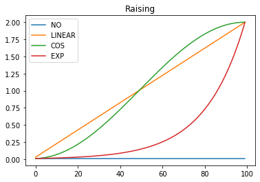
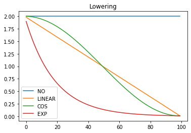
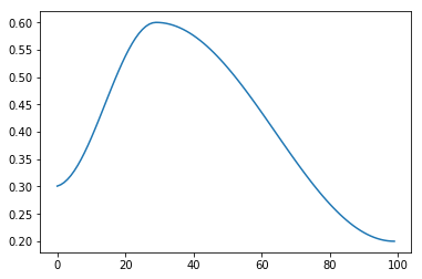
Next we want to define some annealing functions for raising and lowering the learning rate as shown in these plots:
 |
 |
|---|---|
These annealers should take a start and end value and a position between 0 and 1 denoting the relative position in the schedule. Rather than writing a function that takes all 3 of these arguments, when 2 of them are constant, we could either implement the annealing functions as an abstract base class or just use partial functions. Here partial functions are used:
def annealer(f):
    def _inner(start, end):
        return partial(f, start, end)
    return _inner

@annealer
def sched_lin(start, end, pos):
    return start + pos*(end-start)

@annealer
def sched_cos(start, end, pos):
    return start + (1 + math.cos(math.pi*(1-pos))) * (end-start) / 2
@annealer
def sched_no(start, end, pos):
    return start
@annealer
def sched_exp(start, end, pos):
    return start * (end/start) ** pos

def cos_1cycle_anneal(start, high, end):
    return [sched_cos(start, high), sched_cos(high, end)]
annearler is a decorator function. Decorators take a function and return another function and have the fancy @decorator syntax in Python.
We want to combine raising and lowering schedules in a single function alongside a list of positions for when the different schedules start. This is the combine_scheds function:
def combine_scheds(pcts, scheds):
    assert sum(pcts) == 1.
    pcts = tensor([0] + listify(pcts))
    assert torch.all(pcts >= 0)
    pcts = torch.cumsum(pcts, 0)
    def _inner(pos):
        idx = (pos >= pcts).nonzero().max()
        actual_pos = (pos-pcts[idx]) / (pcts[idx+1]-pcts[idx])
        return scheds[idx](actual_pos)
    return _inner

sched = combine_scheds([0.3, 0.7], [sched_cos(0.3, 0.6), sched_cos(0.6, 0.2)])
Which gives the following schedule:
Now we can make our list of callbacks and run the training loop:
cbs = [Recorder(),
       AvgStatsCallback(accuracy),
       ParamScheduler('lr', sched)]
learn = create_learner(get_model_func(0.3), loss_func, data)
run = Runner(cbs=cbs)
run.fit(3, learn)
We can then check the Recorder plots to see if it worked:
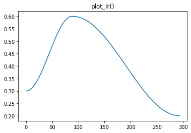 |
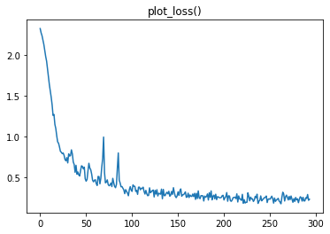 |
|---|---|
Super!
Q & A
-
Why do we have to zero out our gradients in PyTorch?
In models, Parameters often have lots of sources of gradients. The
gradstored by the parameters in PyTorch is a running sum - it is updated with+=, not=. If we didn’t zero the gradients after every update then these old values from previous batches would accumulate. -
Why does the optimizer separate
stepandzero_grad?If we merged the two, we remove the ability to not zero the gradients here. There are cases where we may want that control. For example, what if we are dealing with super resolution 4K images and we can only fit a batch size of 2 into RAM. The stability you get from this batch size is poor and you need a larger batch size. We could instead not zero the grads every time, rather do it ever other batch. Our effective batch size would have then doubled. That’s called gradient accumulation.
-
What’s the difference between FastAI callbacks and PyTorch Hooks?
PyTorch hooks allow you to hook into the internals of your model. So if you want to look at the forward pass of layer 2 of you model, FastAI callbacks couldn’t do that because they are operating at a higher level. All FastAI sees is the forward and backward passes of your model. What goes on within them is PyTorch’s domain.
Links and References
- Lecture video: Lesson9
- Course notebooks: 04_callbacks.ipynb, 05_anneal.ipynb
- Lesson notes by @Lankinen are great transcriptions of the lecture.
- An even deeper dive into PyTorch’s classes, written by the FastAI team: What is torch.nn really?
-
Sylvain’s talk, An Infinitely Customizable Training Loop (from the NYC PyTorch meetup) and the slides that go with it
- Softmax vs Sigmoid? tl;dr sigmoid is a special case of softmax.
- Some other cool Log tricks: Exp-normalize trick, Gumbel-max trick