Fast.ai Lesson 8 Notes: Backprop from the Foundations

Overview

Part 2 of FastAI 2019 is ‘bottom-up’ - building the core of the FastAI library from scratch using PyTorch.

This lesson implements matrix multiplication in pure Python, then refactors and optimizes it using broadcasting and einstein summation. Then this lesson starts to look at the initialization of neural networks. Finally the lesson covers handcoding the forward and backwards passes of a simple model with linear layers and ReLU, before refactoring the code to be more flexible and concise so that you can understand how PyTorch’s work.

Lesson 8 lecture video.

Different Matrix Multiplication Implementations

Naive Matmul

A baseline naive implementation in pure python code:

def matmul(a,b):
    ar,ac = a.shape # n_rows * n_cols
    br,bc = b.shape
    assert ac==br
    c = torch.zeros(ar, bc)
    for i in range(ar):
        for j in range(bc):
            for k in range(ac): # or br
                c[i,j] += a[i,k] * b[k,j]
    return c

Time: 3.26s

Doing loops in pure python and updating array elements one at a time is the bane of performance in python. There is almost always another way that gives better performance. (Though admittedly in some cases the faster way isn’t always obvious or more readable IMHO).

Elementwise Matmul

def matmul(a,b):
    ar,ac = a.shape
    br,bc = b.shape
    assert ac==br
    c = torch.zeros(ar, bc)
    for i in range(ar):
        for j in range(bc):
            # Any trailing ",:" can be removed
            c[i,j] = (a[i,:] * b[:,j]).sum()
    return c

Time: 4.84ms

The loop over k is replaced with a sum() over the elements of row slice in a times the column slice in b. This operation is outsourced to library calls in numpy which are likely compiled code written in C or Fortran, which gives the near 1000x speed-up.

Broadcasting matmul

def matmul(a,b):
    ar,ac = a.shape
    br,bc = b.shape
    assert ac==br
    c = torch.zeros(ar, bc)
    for i in range(ar):
        c[i]   = (a[i  ].unsqueeze(-1) * b).sum(dim=0)
      # c[i]   = (a[i, :, None] * b).sum(dim=0) alternative
    return c

Time: 1.11ms

WTH is this? As is almost always the case, optimizing code comes at the expense of code readability. Let’s work through this to convince ourselves that this is indeed doing a matmul.

Aside: Proof of Broadcasting Matmul

Matmul is just a bunch of dot products between the rows of one matrix and the columns of another: i.e. c[i,j] is the dot product of row a[i, :] and column b[:, j].

Let’s consider the case of 3x3 matrices. a is:

tensor([[1., 1., 1.],
        [2., 2., 2.],
        [3., 3., 3.]], dtype=torch.float64)

b is:

tensor([[0., 1., 2.],
        [3., 4., 5.],
        [6., 7., 8.]], dtype=torch.float64)

Let’s derive the code above looking purely through modifying the shape of a.

1. a has shape (3,3)
2. a[0], first row of a, has shape (3,) and val [1, 1, 1]
3. a[i, :, None] (or a[i].unsqueeze(-1)) has shape (3,1) and val [[1], [1], [1]]

Now multiplying the result of 3 by the matrix b is represented by the expression (I have put brackets in to denote the array dimensions):

From the rules of broadcasting, the $(1)$s on the left array are expanded to match the size of the rows on the right array (size 3). As such, the full expression computed effectively becomes:

The final step is to sum(dim=0), which sums up all the rows leaving a vector of shape (3,), value: [ 9., 12., 15.] . That completes the dot product and forms the first row of matrix c. Simply repeat that for the remaining 2 rows of a and you get the final result of the matmul:

tensor([[ 9., 12., 15.],
        [18., 24., 30.],
        [27., 36., 45.]], dtype=torch.float64)

Einstein Summation Matmul

This will be familiar to anyone who studied Physics, like me! Einstein summation (einsum) is a compact representation for combining products and sums in a general way. From the numpy docs:

“The subscripts string is a comma-separated list of subscript labels, where each label refers to a dimension of the corresponding operand. Whenever a label is repeated it is summed, so np.einsum('i,i', a, b) is equivalent to np.inner(a,b). If a label appears only once, it is not summed, so np.einsum('i', a) produces a view of a with no changes.”

def matmul(a,b): 
    return torch.einsum('ik,kj->ij', a, b)

Time: 172µs

This is super concise with great performance, but also kind of gross. It’s a bit weird that einsum is a mini-language that we pass as a Python string. We get no linting or tab completion benefits that you would get if it were somehow a first class citizen in the language. I think einsum could certainly be great and quite readable in cases where you are doing summations on tensors with lots of dimensions.

PyTorch Matmul Intrinsic

Matmul is already provided by PyTorch (or Numpy) using the @ operator:

def matmul(a, b):
    return a@b

Time: 31.2µs

The best performance is, unsuprisingly, provided by the library implementation. This operation will drop down to an ultra optimized library like BLAS or cuBLAS, written by low-level coding warrior-monks working at Intel or Nvidia who have have spent years hand optimizing linear algebra code in C and assembly. (The matrix multiply algorithm is actually a very complicated topic, and no one knows what the fastest possible algorithm for it is. See this wikipedia page for more). So basically in the real world, you should probably avoid writing your own matmal!

Single Layer Network: Forward Pass

Work through the Jupyter notebook: 02_fully_connected.ipynb

Create simple network for MNIST. One hidden layer and one output layer, parameters:

n = 50000 
m = 784
nout = 1 # just for teaching purposes here, should be 10
nh = 50

The model will look like this:

Linear activation function:

def lin(x, w, b):
    return x@w + b

ReLU activation function:

def relu(x):
    return x.clamp_min(0.)

Loss function we’ll use here is the Mean Squared Error (MSE). This doesn’t quite fit for a classification task, but it’s used as a pedgogical tool for teaching the concepts of loss and backpropagation.

def mse(output, targ):
    return (output.squeeze(-1) - targ).pow(2).mean()

Forward Pass of model:

def model(xb):
    l1 = lin(xb, w1, b1)
    l2 = relu(l1)
    l3 = lin(l2, w2, b2)
    return l3

preds = model(x_train)
loss = mse(preds, y_train)

Let’s go over the tensor dimensions to review how the forward pass works:

• Input $X$ is a batch of vectors of size 784, shape=[N, 784]
• Hidden layer is of size 50 and has an input of shape=[N, 784] => $W_1$: shape=[784, 50], $b_1$: shape=[50], output: shape=[N, 50]
• Output layer has size 1 and input of shape=[N, 50] => $W_2$: shape=[50, 1], $b_2$: shape=[1], output: shape=[N, 1]

Initialisation

Recent research shows that weight initialisation in NNs is actually super important. If the network isn’t initialised well, then after one pass through the network the output can sometimes become vanishingly small or even explode, which doesn’t bode well for when we do backpropagation.

A rule of thumb to prevent this is:

1. The mean of the activations should be zero
2. The variance of the activations should stay close to 1 across every layer.

Let’s try Normal initialisation with a linear layer:

w1 = torch.randn(m,nh)
b1 = torch.zeros(nh)
w2 = torch.randn(nh,1)
b2 = torch.zeros(1)

x_valid.mean(),x_valid.std()
>>> (tensor(-0.0059), tensor(0.9924))

t = lin(x_valid, w1, b1)
t.mean(),t.std()
>>>	(tensor(-1.7731), tensor(27.4169))

After one layer, it’s already in the rough.

A better initialisation is Kaiming/He initialisation (paper). For a linear activation you simply divide by the square root of the number of inputs to the layer.:

w1 = torch.randn(m,nh)/math.sqrt(m)
b1 = torch.zeros(nh)
w2 = torch.randn(nh,1)/math.sqrt(nh)
b2 = torch.zeros(1)

Test:

t = lin(x_valid, w1, b1)
t.mean(),t.std()
>>> (tensor(-0.0589), tensor(1.0277))

The initialisation used depends on the activation function used. If we instead use a ReLU layer then we have to do something different from the linear.

If you have a normal distribution with mean 0 with std 1, but then clamp it at 0, then obviously the resulting distribution will no longer have mean 0 and std 1.

From pytorch docs: a: the negative slope of the rectifier used after this layer (0 for ReLU by default)

\[\text{std} = \sqrt{\frac{2}{(1 + a^2) \times \text{fan_in}}}\]

This was introduced in the paper that described the Imagenet-winning approach from He et al: Delving Deep into Rectifiers, which was also the first paper that claimed “super-human performance” on Imagenet (and, most importantly, it introduced resnets!)

w1 = torch.randn(m,nh)*math.sqrt(2/m)

Test:

t = relu(lin(x_valid, w1, b1))
t.mean(),t.std()
>>> (tensor(0.5854), tensor(0.8706))

The function that does this in the Pytorch library is:

from torch.nn import init

w1 = torch.zeros(m,nh)
init.kaiming_normal_(w1, mode='fan_out')

'fan_out' means that we divide by m, while 'fan_in' would mean we divide by nh. This bit here is confusing because we are using the opposite convention to PyTorch has. PyTorch Linear layer stores the matrix as (nh, m), where our implementation is (m, nh). Looking inside the forward pass of linear in PyTorch the weight matrix is transposed before being multiplied. This means that for this special case here we swap ‘fan_out’ and ‘fan_in’. If we were using PyTorch’s linear layer we’d initialize with ‘fan_in’.

Let’s get a better view of the means and standard deviations of the model with Kaiming initialization by running the forward pass a few thousand times and looking at the distributions.

(Update, 8/2/20: Old plots were buggy. Fixed plots, added code, and added plots with Linear-ReLU model).

Linear-ReLU Model, Kaiming Init

def model_dist(x):
    w1 = torch.randn(m, nh) * math.sqrt(2/m)
    b1 = torch.zeros(nh)
    
    l1 = lin(x, w1, b1)
    l2 = relu(l1)
    l2 = l2.detach().numpy()
    return l2.mean(), l2.std()

data = np.array([model_dist(x_train) for _ in range(3000)])
means, stds = data[:, 0], data[:, 1]

Mean and standard deviations of the outputs with Kaiming Initialization:

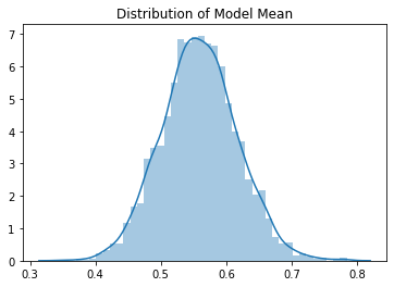
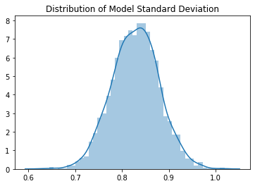
The means and standard deviations of the output have Gaussian distributions. The mean of the means is 0.55 and the mean of the standard deviations is 0.82. The mean is shifted to be positive because the ReLU has set all the negative values to 0. The typical standard deviation we get with Kaiming initialization is quite close to 1, which is what we want.

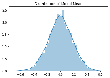
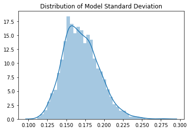
Full Model, Kaiming Init

def model_dist(x):
    w1 = torch.randn(m, nh) * math.sqrt(2/m)
    b1 = torch.zeros(nh)
    w2 = torch.randn(nh, nout) / math.sqrt(nh)
    b2 = torch.zeros(nout)
    
    l1 = lin(x, w1, b1)
    l2 = relu(l1)
    l3 = lin(l2, w2, b2)
    l3 = l3.detach().numpy()
    return l3.mean(), l3.std()

data = np.array([model_dist(x_train) for _ in range(3000)])
means, stds = data[:, 0], data[:, 1]

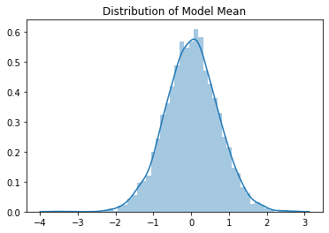
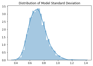
The means have a clearly Gaussian distribution with mean value 0.01. The standard deviations have a slightly skewed distribution, but the mean value is 0.71. We see empirically that the expected output values of the model after Kaiming initialisation are approximately mean 0, standard deviation near to 1, so it seems to be working well.

Aside: Init in Pytorch - sqrt(5)??

In torch.nn.modules.conv._ConvNd.reset_parameters:

def reset_parameters(self):
    init.kaiming_uniform_(self.weight, a=math.sqrt(5))
    if self.bias is not None:
        fan_in, _ = init._calculate_fan_in_and_fan_out(self.weight)
        bound = 1 / math.sqrt(fan_in)
        init.uniform_(self.bias, -bound, bound)

A few differences here:

1. Uses Uniform distribution instead of a Normal distribution. This just seems to be convention the PyTorch authors have chosen to use. Not an issue and it is centred around zero anyway.
2. The sqrt(5) is probably a bug, according to Jeremy.

The initialization for the linear layer is similar.

From the documentation on parameter a:

a: the negative slope of the rectifier used after this layer (0 for ReLU by default)

For ReLU it should be 0, but here it is hard-coded to sqrt(5). So for ReLU activations in Conv layers, the initialization of some layers in PyTorch is suboptimal by default.

(Update 8/2/20). We can look at the distribution of the outputs of our model using PyTorch’s default init:

def model_dist(x, n_in, n_out):
    layers = [nn.Linear(n_in, nh),
              nn.ReLU(),
              nn.Linear(nh, n_out)]
    for l in layers:
        x = l(x)
    x = x.detach().numpy()
    return x.mean(), x.std()

Mean value is approximately 0.0 and the standard deviation is 0.16. This isn’t great - we have lost so much variation after just two layers. The course investigates this more in the notebook: 02a_why_sqrt5.ipynb.

(Update: Here is a link to the issue in PyTorch, still open (2020-2-13), https://github.com/pytorch/pytorch/issues/18182)

Gradients and Backpropagation

To understand backpropagation we need to first understand the chain rule from calculus. The model looks like this:

Where $L$ denotes the loss. We can also write this as:

Or fully expanded:

In order to update the parameters of the model, we need to know what is the gradient of $L$ with respect to (wrt) the parameters of the model. What are the parameters of this model? They are: $W_{ij}^{(1)}$, $W^{(2)}_{ij}$, $b^{(1)}_i$, $b^{(2)}_i$ (including indices to remind you of the tensor rank of the parameters). The partial derivatives of the parameters we want to calculate are:

On first sight, looking at the highly nested function of $L$ finding the derivative of it wrt to matrices and vectors looks like a brutal task. However the cognitive burden is greatly decreased thanks to the chain rule.

When you have a nested function, such as:

The chain rule tells you that the derivative of $f$ wrt to $x$ is:

A helpful mnemonic is to picture the $\partial q$’s ‘cancelling out’.

Backpropagation: Graph Model

How does this fit into backpropagation? Things become clearer when the model is represented as a computational graph, instead of as equations.

Imagine some neuron $f$ in the middle of a bigger network. In the forward pass, data $x$ and $y$ flows from left to right through the neuron $f$, outputting $z$, then calculating the loss $L$. Then we want the gradients of all the variables wrt the loss. Here is a diagram taken from CS231 course :

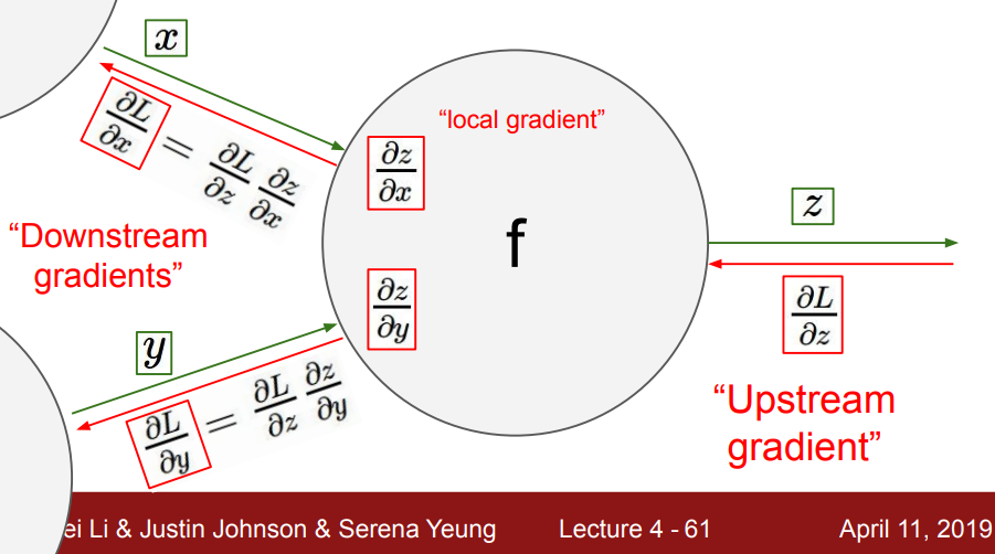
(Source: brilliant CS231 course from Stanford. This lecture made backpropagation ‘click’ for me: video, notes).

Calculate the gradients of the variables backwards from right to left. We have the gradient $\frac{\partial L}{\partial z}$ coming from ‘upstream’. To calculate $\frac{\partial L}{\partial x}$, we use the chain rule:

The gradient = upstream gradient $\times$ local gradient. This relation recurses back through the rest of the network, so a neuron directly before $x$ would receive the upstream gradient $\frac{\partial L}{\partial x}$. The beauty of the chain rule is that it enables us to break up the model into its constituent operations/layers, compute their local gradients, then multiply by the gradient coming from upstream, then propagate the gradient backwards, repeating the process.

Coming back to our model - $\mbox{MSE}(\mbox{Lin2}(\mbox{ReLU}(\mbox{Lin1(x)})), y)$ - to compute the backward pass we just need to compute the expressions for the derivatives of MSE, Linear layer, and ReLU layer.

Gradients of Vectors or Matrices

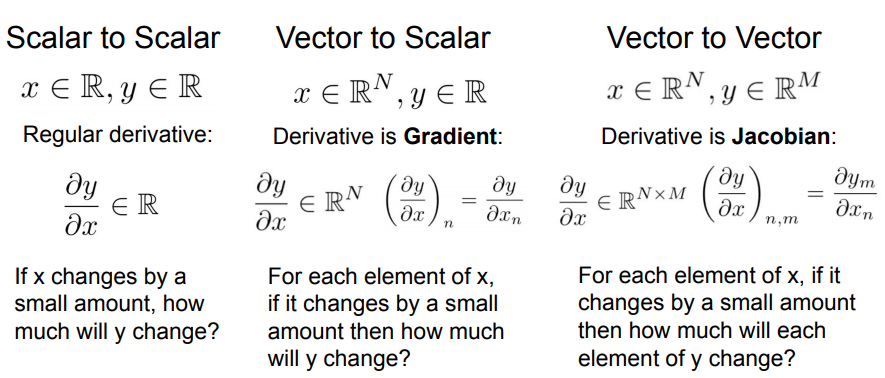
What happens when $z$, $x$, and $y$ aren’t scalar, but are vectors or matrices? Nothing changes with how backpropagation works - just the maths for computing the local gradients gets a bit hairier.

If the loss $L$ is a scalar and $\mathbf{z}$ is a vector then the derivative would be vector:

Think: “For each element of $\mathbf{z}$, if it changes by a small amount how much will $L$ change?”

If $\mathbf{x}$ and $\mathbf{z}$ are both vectors then the derivative would be a Jacobian matrix:

Think: “For each element of $\mathbf{x}$”, if it changes by a small amount then how much will each element of $\mathbf{y}$ change?

Summary, again taken from CS231n:

More info: a full tutorial on matrix calculus is provided here: Matrix Calculus You Need For Deep Learning.

Gradient of MSE

The mean squared error:

Where $N$ is the batch size, $z_i$ is the output of the model for data point $i$, and $y_i$ is the target value of $i$. The loss is the average of the squared error in a batch. $\mathbf{z}$ is a vector here. The derivative of scalar $L$ wrt a vector will be vector.

All the other terms in the sum go to zero because they don’t depend on $z_i$. Notice also how $L$ doesn’t appear in the gradient - we don’t actually need the value of the loss in the backwards step!

In Python code:

def mse_grad(inp, targ):
    # inp from last layer of model, shape=(N,1)
    # targ targets, shape=(N)
    # want: grad of MSE wrt inp, shape=(N, 1)
    grad = 2. * (inp.squeeze(-1) - targ).unsqueeze(-1) / inp.shape[0]
    inp.g = grad

Gradient of Linear Layer

Linear layer:

Need to know:

Where $X$, and $W$ are matrices and $b$ is a vector. We already know $\frac{\partial L}{\partial Y}$ - it’s the upstream gradient (remember it’s a tensor, not necessarily a single number).

Here is where the maths gets a bit hairier. It’s not worth redoing the derivations of the gradients here, which can be found in these two sources: matrix calculus for deep learning, linear backpropagation.

The results:

In Python:

def lin_grad(inp, out, w, b):
    # inp - incoming data (x)
    # out - upstream data 
    # w - weight matrix
    # b - bias
    inp.g = out.g @ w.t()
    w.g = inp.t() @ out.g
    b.g = out.g.sum(dim=0)

Gradient of ReLU

Gradient of ReLU is easy. For the local gradient - if the input is less than 0, gradient is 0, otherwise it’s 1. In Python

def relu_grad(inp, out):
    # inp - input (x)
    # out - upstream data
    inp.g = (inp>0).float() * out.g

Putting it together: forwards and backwards

def forwards_and_backwards(inp, targ):
    # forward pass
    l1 = lin(inp, w1, b1)
    l2 = relu(l1)
    out = lin(l2, w2, b2)
    loss = mse(out, targ)
    
    # backward pass
    mse_grad(out, targ)
    lin_grad(l2, out, w2, b2)
    relu_grad(l1, l2)
    lin_grad(inp, l1, w1, b1)

Check the Dimensions. How does batchsize affect things?

(Added 17-03-2020)

What do the dimensions of the gradients look like? The loss $L$ is a scalar and the parameters are tensors so remembering the rules above the derivative of $L$ wrt any parameter will have the same dimensionality as that parameter. The gradients of the parameters have the same shape as the parameters, which makes intuitive sense.

• w1.g.shape => [784, 50]
• b1.g.shape => [50]
• w2.g.shape => [50, 1]
• b2.g.shape => [1]
• loss.shape => [] (scalar)

Notice how the batch size doesn’t appear in the gradients. That’s not to say it doesn’t matter - the batch size is there behind the scenes in the gradient calculation: the loss is an average of the individual losses in a batch, and also as a dimension multiplied out in the matrix multiplies of the gradient calculations.

To be even more explicit with the dimensions:

inp.g = out.g @ self.w.t()		# [N, 784] = [N, 50] @ [50, 784]
self.w.g = inp.t() @ out.g		# [784, 50] = [784, N] @ [N, 50]
self.b.g = out.g.sum(0)			# [50] = [N, 50].sum(0)

inp.g = out.g @ self.w.t()		# [N, 50] = [N, 1] @ [1, 50]
self.w.g = inp.t() @ out.g		# [50, 1] = [50, N] @ [N, 1]
self.b.g = out.g.sum(0)			# [1] = [N, 1].sum(0)

With bigger batch size you are accumulating more gradients because it is basically doing more dot products. If you could hack the loss so its gradient is constant and increase the batch size then these gradients would get correspondingly larger (in absolute size).

In reality this is cancelled out because the larger the batch size the smaller the gradient. You can see this by look at the gradient calculation for MSE: it is divided by the batch size.

Let’s vary the batchsize and plot the average gradients of the parameters W1 and W2, alongside the loss and loss gradient:

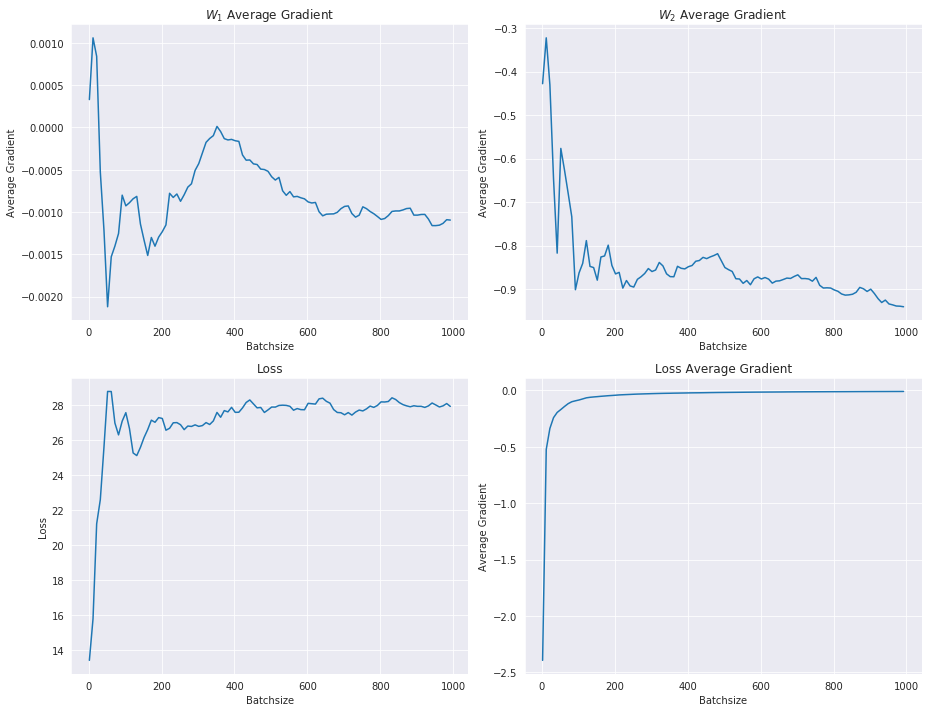
The average gradient of the loss gets smaller with increasing batchsize, while the other gradients and the loss pretty much settle towards some value.

Refactoring

(Updated 17-03-2020)

The rest of the notebook - 02_fully_connected.ipynb - is spent refactoring this code using classes so we understand how PyTorch’s classes are constructed. I won’t reproduce it all here. If you want to reproduce it yourself you need to create a base Module that all your layer inherit from, which remembers the inputs it was called with (so it can do gradient calculations):

class Module():
    def __call__(self, *args):
        self.args = args
        self.out = self.forward(*args)
        return self.out
    
    def forward(self): raise Exception('not implemented')
    def backward(self): self.bwd(self.out, *self.args)

The different layers (linear, ReLU, MSE) need to subclass Module and implement forward and bwd methods.

The end result of this gives an equivalent implementation of PyTorch’s nn.Module. The equivalent with PyTorch classes, which we can now use, is:

from torch import nn


class Model(nn.Module):
    def __init__(self, n_in, n_out):
        super().__init__()
        self.layers = [nn.Linear(n_in, nh), nn.ReLU(), nn.Linear(nh, n_out)]
        self.loss = mse
    def __call__(self, x, targ):
        for l in self.layers:
            x = l(x)
        return self.loss(x.squeeze(), targ)

Now that we understand how backprop works, we luckily don’t have to derive anymore derivatives of tensors, we can instead from now on harness PyTorch’s autograd to do all the work for us!

model = Model(m, nh, 1)
loss = model(x_train, y_train)
loss.backward() # do the backward pass!

Links and References

• Lesson 8 lecture video.

• Lesson notes from Laniken provide a transcription of the lesson.

• Broadcasting tutorial from Jake Vanderplas: Computation on Arrays: Broadcasting.

• Deeplearning.ai notes on initialisation with nice demos of different initialisations and their effects: deeplearning.ai

• Kaiming He paper on initialization with ReLu activations (assignment: read section 2.2 of this paper): Delving Deep into Rectifiers: Surpassing Human-Level Performance on ImageNet Classification

• Fixup Initialization: paper where they trained a 10,000 layer NN with no normalization layers through careful initialization.

• Things that made Backprop ‘click’ for me:

  • CS231: backpropagation explained using the a circuit model: http://cs231n.github.io/optimization-2/
  • CS231: backpropagation lecture (Andrej Karpathy), slides.
  • Blog post with worked examples of backpropagation on simple calculations.
  • Calculus on Computational Graphs, Chris Olah.

• StackExchange: Tradeoff batch size vs. number of iterations to train a neural network - worth reading about somewhat unintuitive effect batchsize has on training performance and speed.