In this post I explore Stochastic Gradient Descent (SGD) which is an optimization method commonly used in neural networks. This continues Lesson 2 of fast.ai on Stochastic Gradient Descent (SGD). I will copy from the fast.ai notebook on SGD and dig deeper into the what’s going on there.
Linear Regression
We will start with the simplest model - the Linear model. Mathematically this is represented as:
\[\vec{y} = X \vec{a} + \vec{b}\]Where $X$ is a matrix where each of the rows is a data point, $\vec{a}$ is the vector of model weights, and $\vec{b}$ is a bias vector. In the 1D case, these would correspond to the familiar ‘slope’ and ‘intercept’ of a line. We can make this more compact by combining the bias inside of the model weights and adding an extra column to $X$ with all values set to one. These are represented in Pytorch as tensors.
In Pytorch, a tensor is a data structure that encompasses arrays of any dimension. A vector is a tensor of rank 1, while a matrix is a tensor of rank 2. For simplicity we will stick to the case of a 1D linear model. In PyTorch $X$ would then be:
n=100
x = torch.ones(n,2)
x[:,0].uniform_(-1.,1)
The model has two parameters and there are n=100 datapoints. x therefore has shape (100, 2). The .uniform_(-1., 1) generates floating point numbers between -1 and 1. The trailing _ is PyTorch convention that the function operates inplace.
Let’s look at the first 5 values of x:
> x[:5]
tensor([[ 0.7893,  1.0000],
        [-0.7556,  1.0000],
        [-0.0055,  1.0000],
        [-0.2465,  1.0000],
        [ 0.0080,  1.0000]])
Notice how the second column is all 1s - this is the bias.
We’ll now set the true values for the model weights, $a$, to slope=3 and intersection=10:
a = tensor(3.,10)
a_true = a
With x and a set we can now generate some fake data with some small normally distributed random noise:
y = x@a + torch.randn(n) * 0.6
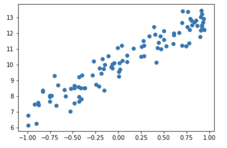
Loss Function
We want to find parameters (weights) a such that they minimize the error between the points and the line x@a. Note that here a is unknown. For a regression problem the most common error function or loss function is the mean squared error. In python this function is:
def mse(y_hat, y):
    return ((y_hat-y)**2).mean()
Where y is the true value and y_hat is the predicted value.
We start with guess at the value of the weights a:
a = tensor(-1, 1)
We can make prediction for y, y_hat, and compute the error against the known values:
> y_hat = x@a
> mse(y_hat, y)
tensor(92.9139)
So far we have specified the model (linear regression) and the evaluation criteria (or loss function). Now we need to handle optimization; that is, how do we find the best values for a? How do we find the best fitting linear regression.
Gradient Descent
We would like to find the values of a that minimize mse_loss. Gradient descent is an algorithm that minimizes functions. Given a function defined by a set of parameters, gradient descent starts with an initial set of parameter values and iteratively moves toward a set of parameter values that minimize the function. This iterative minimization is achieved by taking steps in the negative direction of the function gradient. Here is gradient descent implemented in PyTorch:
a = nn.Parameter(a)
lr = 1e-1

def update():
    y_hat = x@a
    loss = mse(y, y_hat)
    loss.backward()
    with torch.no_grad():
      	# don't compute the gradient in here
        a.sub_(lr * a.grad)
        a.grad.zero_()

for t in range(100):
  update()
We are going to create a loop. We’re going to loop through 100 times, and we’re going to call a function called update. That function is going to:
- Calculate
y_hat(i.e. our prediction) - Calculate loss (i.e. our mean squared error)
- Calculate the gradient. In PyTorch, calculating the gradient is done by using a method called
backward. Mean squared error was just a simple standard mathematical function. PyTorch keeps track of how it was calculated and lets us automatically calculate the derivative. So if you do a mathematical operation on a tensor in PyTorch, you can callbackwardto calculate the derivative and the derivative gets stuck inside an attribute called.grad. - Then take the weights
aand subtract the gradient from them (sub_). There is an underscore there because that’s going to do it in-place. It’s going to actually update those coefficientsato subtract the gradients from them. Why do we subtract? Because the gradient tells us if the whole thing moves downwards, the loss goes up. If the whole thing moves upwards, the loss goes down. So we want to do the opposite of the thing that makes it go up. We want our loss to be small. That’s why we subtract. lris our learning rate. All it is is the thing that we multiply by the gradient.
Animate it!
Here is an animation of the training gradient descent with learning rate LR=0.1

Notice how it seems to spring up to find the intercept first then adjusts to get the slope right. The starting guess at the intercept is 1, while the real value is 10. At the start this would cause the biggest loss so the we would expect the gradient on the intercept parameter to be higher than the gradient on the slope parameter.
It sucessfully recovers, more or less, the weights that we generated the data with:
> a
tensor([3.0332, 9.9738]
Stochastic Gradient Descent
The gradient descent algorithm calculates the loss across the entire dataset every iteration. For this problem this works great, but it won’t scale. If we were training on imagenet then we’d have to compute the loss on 1.5 million images just to do a single update of the parameters. This would be both incredibly slow and also impossible to fit into computer memory. Instead we grab random mini-batches of 64, or so, data points and compute the loss and gradient with those and then update the weights. As code this looks almost identical to before, but with some random indexes added to x and y:
def update_mini(rand_idx):
    y_hat = x[rand_idx]@a
    loss = mse(y[rand_idx], y_hat)
    loss.backward()
    with torch.no_grad():
        a.sub_(lr * a.grad)
        a.grad.zero_()
Using mini-batches approximates the gradient, but also adds random noise to the optimiser causing the parameters to ‘jump around’ a little. This can make it require more iterations to converge. We will see this visually in the next section. On the other hand, some random noise is a good thing in training neural networks because it allows the optimiser to better explore the high dimensional parameter space and potentially find a solution with a lower loss.
Animate it!
Here is an animation of the training with batch size of 16:
It converges on the same answer as gradient descent, but it is a little slower and has a bit of jitter that isn’t in the gradient descent animation.
Experiments with the Learning Rate and Batch Size
We can gain a better understanding of how SGD works by playing with the parameters, learning rate and batch size, and visualising the learning process.
Learning Rate
Here the learning rate in SGD is varied, keeping the batch size fixed at 16.
| Parameters | Animation |
|---|---|
SGD LR=1e-2bs=16 |
 |
SGD LR=1e-1bs=16 |
|
SGD LR=1.0 bs=16 |
 |
With the learning rate of 0.01 it too small and it takes an age, but it does eventually converge on the right answer. With a learning rate of 1.0 the whole thing goes off the rails and it can’t get anywhere near the right answer.
Batch Size
Here the batch size in SGD is varied, holding the learning rate fixed at LR=0.1:
| Parameters | Animation |
|---|---|
SGD bs=1 |
 |
SGD bs=2 |
 |
SGD bs=4 |
 |
SGD bs=8 |
 |
SGD bs=16 |
|
SGD bs=32 |
 |
SGD bs=64 |
 |
All of the instances do converge to the right answer in this case (though in general that wouldn’t be the case for all problems). For bs=1 it jumps around a lot even after it gets into the right place. This is because the weights are updated using only one data point every iteration. So it jitters around the right solution and will never stop jittering with more iterations.
However with increasing batch size the jitter gets less and less. At batch size of 64 the animation is almost identical to the gradient descent animation. This makes sense since n=100 so with bs=64 we have almost gone back to the full gradient descent algorithm (which would be bs=n ).
References
- FastAI Lesson 2 lecture: https://course.fast.ai/videos/?lesson=2
- FastAI Lesson 2 notes: https://github.com/hiromis/notes/blob/master/Lesson2.md
- FastAI SGD from Scratch notebook: https://github.com/fastai/course-v3/blob/master/nbs/dl1/lesson2-sgd.ipynb