
Overview of Lesson
This lesson firstly dives deeper in to fastai’s approach to loading data for deep learning: the data block API; and secondly goes into more advanced problems beyond classification that you can solve with deep learning and the fastai library. Namely:
- Multi-label classification (Planet Amazon dataset)
- Regression problems (Head Orientation dataset)
- Image Segmentation (Camvid dataset)
- Text Classification (IMDB dataset)
The lesson ends with a brief look at the fundamentals of deep learning: non-linearity and the Universal Approximation theorem.
DataBlock API
The trickiest step previously in deep learning has often been getting the data into a form that you can get it into a model. So far we’ve been showing you how to do that using various “factory methods” which are methods where you say, “I want to create this kind of data from this kind of source with these kinds of options.” That works fine, sometimes, and we showed you a few ways of doing it over the last couple of weeks. But sometimes you want more flexibility, because there’s so many choices that you have to make about:
- Where do the files live
- What’s the structure they’re in
- How do the labels appear
- How do you spit out the validation set
- How do you transform it
In fastai there is this unique API called the data block API. The data block API makes each one of those decisions a separate decision that you make. There are separate methods with their own parameters for every choice that you make around how to create / set up the data.
To give you a sense of what that looks like, the first thing I’m going to do is go back and explain what are all of the PyTorch and fastai classes you need to know about that are going to appear in this process. Because you’re going to see them all the time in the fastai docs and PyTorch docs.
We will now explain the different PyTorch and fastai classes that appear in the data block API.
Dataset (PyTorch)
The first class you need to know is the Dataset class, which is part of PyTorch. It is very simple, here is the source code:

It actually does nothing at all. It is an abstract class, defining that subclasses of Dataset must implement __getitem__ and __len__ methods. The first means you can use the python array indexing notation with a Dataset object: d[12]; and the second means that you can get the length of the Dataset object: len(d).
DataLoader (PyTorch)
A Dataset is not enough to train a model. For SGD we need to be able to produce mini-batches of data for training. To create mini-batches we use another PyTorch class called a DataLoader. Here is the documentation for that:

- This takes a
Datasetas a parameter. - It will create batches of size
batch_sizeby grabbing items at random from the dataset. - The dataloader then sends the batch over to the GPU to your model.
DataBunch (fastai)
The DataLoader is still not enough to train a model. To train a model we need to split the data into training, validation, and testing. So for that fastai has its own class called DataBunch.

The DataBunch combines together a training DataLoader, a validation DataLoader, and optionally a test DataLoader.
You can read from the documentation that DataBunch also handles on-the-fly data transformations with tfms and allows you to create a custom function for building the mini-batches with collate_fn.
Learn to use the data block API by example
I won’t reproduce the examples here because fastai’s documentation already has a fantastic page full of data block API examples here. I recommend you read the whole thing or download and run it because the documentation pages are all Jupyter notebooks!
Image Transforms (docs)
- fastai provides a complete image transformation library written from scratch in PyTorch. Although the main purpose of the library is data augmentation for use when training computer vision models, you can also use it for more general image transformation purposes.
- Data augmentation is perhaps the most important regularization technique when training a model for Computer Vision: instead of feeding the model with the same pictures every time, we do small random transformations (a bit of rotation, zoom, translation, etc…) that don’t change what’s inside the image (to the human eye) but do change its pixel values. Models trained with data augmentation will then generalize better.
get_transformscreates a list of a image transformations.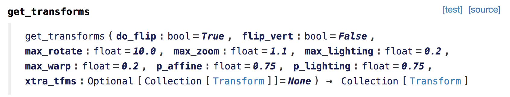
- Which image transformations are appropriate to use depends on your problem and what would likely appear in the real data. Flipping images of cats/dogs vertical isn’t useful because they wouldn’t appear upside-down. While for satellite images it makes no sense to zoom, but flipping them vertically and horizontally would make sense.
- fastai is unique in that it provides a fast implementation of perspective warping. This is the
max_wapoption inget_transforms. This is like the kind of warping that occurs if you take a picture of a cat from above versus from below. This kinds of transformation wouldn’t make sense for satellite images, but would for cats and dogs.
Planet Amazon: Multi-label Classification
(Link to Notebook)
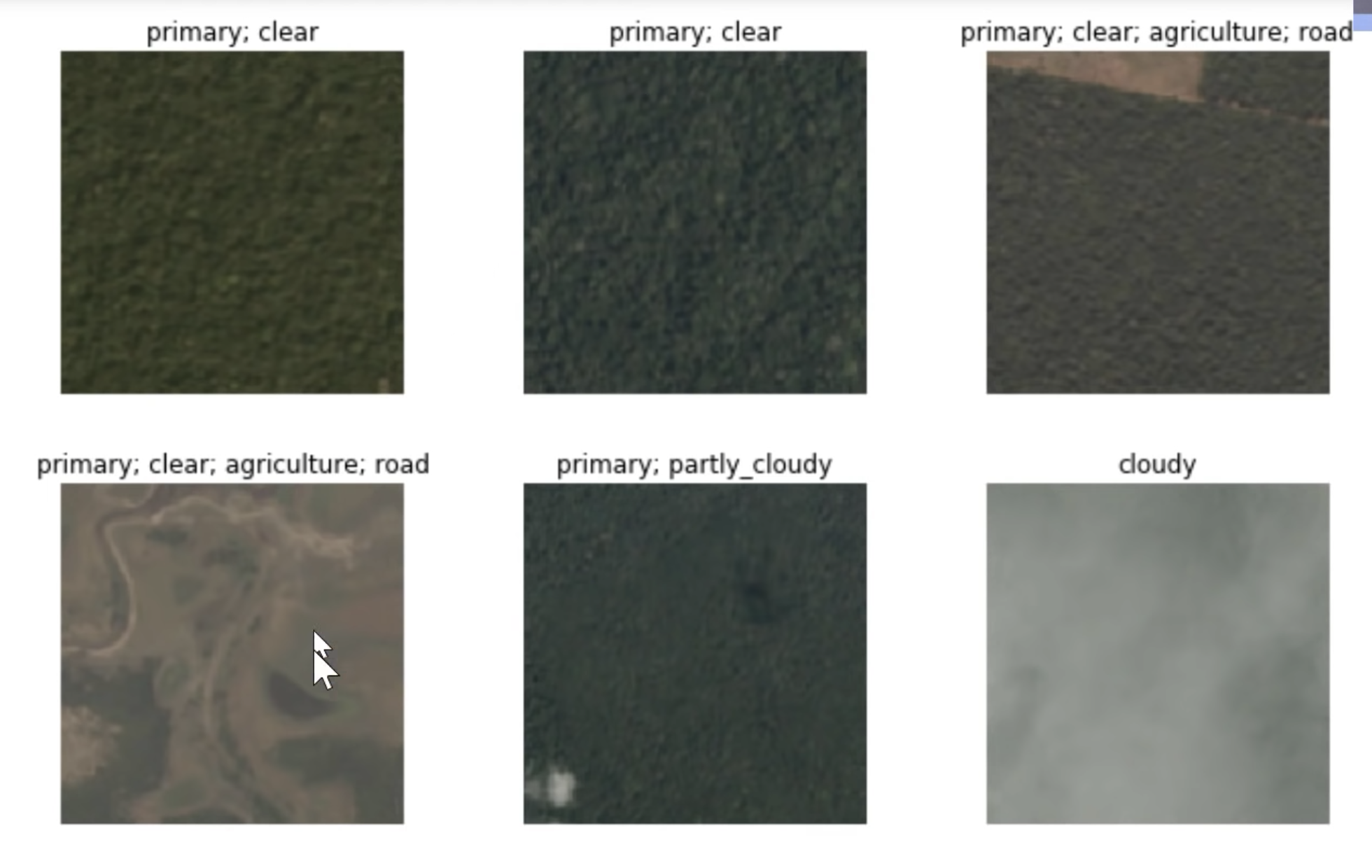
The Planet Amazon dataset is an example of a multi-label classification problem. The dataset consists of satellite images taken of the Amazon rainforest, each of which has a list of labels describing what’s in the image, for example: weather, trees, river, agriculture.
Here is a sample of the images:
Here is what some of the training labels look like:
df = pd.read_csv(path/'train_v2.csv')
df.head()
| image_name | tags | |
|---|---|---|
| 0 | train_0 | haze primary |
| 1 | train_1 | agriculture clear primary water |
| 2 | train_2 | clear primary |
| 3 | train_3 | clear primary |
| 4 | train_4 | agriculture clear habitation primary road |
There are many different labels that an image can have and so there are a huge number of combinations. This makes treating it as a single label classification impractical. If there were 20 different labels then there could be as many as $2^{20}$ possible combinations. Better to have the model output a 20d vector than have it try to learn $2^{20}$ individual labels!
Loading the Data
Code for loading data with comments:
tfms = get_transforms(flip_vert=True, max_lighting=0.1, max_zoom=1.05, max_warp=0.)

src = (ImageList.from_csv(path, 'train_v2.csv', folder='train-jpg', suffix='.jpg')
       # image names are listed in a csv file (names found by default in first column)
       # path to the data is `path`
       # the folder containing the data is `folder`
       # the file ext is missing from the names in the csv so add `suffix` to them.
       .split_by_rand_pct(0.2)
       # split train/val randomly with 80/20 split
       .label_from_df(label_delim=' ')
       # label from dataframe (the output of `from_csv`). Default is second column.
       # split the tags by ' '
      )

data = (src.transform(tfms, size=128)
        .databunch().normalize(imagenet_stats))
Create the Model
To create a Learner for multi-label classification you don’t need to do anything different from before. fastai create_cnn takes the DataBunch object and see that the type of the target variable and takes care of creating the output layers etc for you behind the scenes.
For this particular problem the only thing we do different is to pass a few different metrics to the Learner.
acc_02 = partial(accuracy_thresh, thresh=0.2)
f_score = partial(fbeta, thresh=0.2)
learn = cnn_learner(data, models.resnet50, metrics=[acc_02, f_score])
Note: metrics change nothing about how the model learns. They are only an output for you to see how well it is learning. They are not to be confused with the model’s loss function.
What are these metrics about here? Well the network will output some M-dimensional vector with numbers between 0 and 1. Each of the the elements in this vector indicate the presence of one of the labels, but we need to decide a threshold value, above which we will say that this or that label is ‘on’. We set this threshold to 0.2. acc_02 and f_score here are the accuracy and f-score after applying 0.2 thresholding to the model output.
Train the Model
The model is trained in the basically same way as in the previous lessons:
- Freeze all the layers except the head.
- Run
lr_find(). - Train the head for a few cycles.
- Unfreeze the rest of the network and run
lr_find()again. - Train the whole model for some more cycles with a differential learning rate.
After this however, Jeremy shows a cool new trick however called progressive resizing. Here you train your network on images that are smaller, then continue training the network on larger images. So start $128^2$ for a few cycles, then $256^2$, $512^2$ etc. You can save time on training for higher resolution images by effectively using smaller resolution models as pretrained models for larger resolutions.
To do this you simply have to tweak the DataBunch from before and give it a new size then give that to the Learner:
data = (src.transform(tfms, size=256)
        .databunch().normalize(imagenet_stats))

learn.data = data
data.train_ds[0][0].shape
I won’t reproduce anymore here, but the full example is covered in this Lesson 3 homework notebook.
Camvid: Image Segmentation
(Link to Notebook)
The next example we’re going to look at is this dataset called CamVid. It’s going to be doing something called segmentation. We’re going to start with a picture like the left and produce a colour-coded picture on the right:
| Input Image | Segmented Output |
|---|---|
 |
 |
All the bicycle pixels are the same colour, all the car pixels are the same color etc.
-
Segmentation is an image classification problem where you need to label every single pixel in the image.
-
In order to build a segmentation model, you actually need to download or create a dataset where someone has actually labeled every pixel. As you can imagine, that’s a lot of work, so you’re probably not going to create your own segmentation datasets but you’re probably going to download or find them from somewhere else.
-
We use Camvid dataset. fastai comes with many datasets available for download through the fastai library. They are listed here.
Loading the Data
- Segmentation problems come with sets of images: the input image and a segmentation mask.
- The segmentation mask is a 2D array of integers.
- fastai has a special function for opening image masks called
open_mask. (For ordinary images useopen_image).
Create a databunch:
codes = np.loadtxt(path/'codes.txt', dtype=str)

get_y_fn = lambda x: path_lbl/f'{x.stem}_P{x.suffix}'

src = (SegmentationItemList.from_folder(path_img)
       #Where to find the data? -> in path_img and its subfolders
       .split_by_fname_file('../valid.txt')
       #How to split in train/valid? -> using predefined val set in valid.txt
       .label_from_func(get_y_fn, classes=codes)
       #How to label? -> use the label function on the file name of the data
      )

data = (src.transform(get_transforms(), tfm_y=True, size=128)
        #Data augmentation? -> use tfms with a size of 128,
        # also transform the label images (tfm_y)
        .databunch(bs=8)
        #Finally -> use the defaults for conversion to databunch
       ).normalize(imagenet_stats)
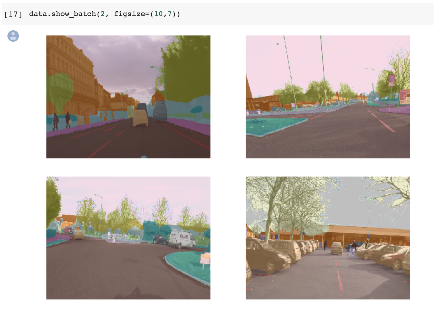
fastai shows the images with the masks superimposed for you with show_batch:
Create the Model
- For segmentation an architecture called UNET turns out to be better than using a CNN. Here’s what it looks like:
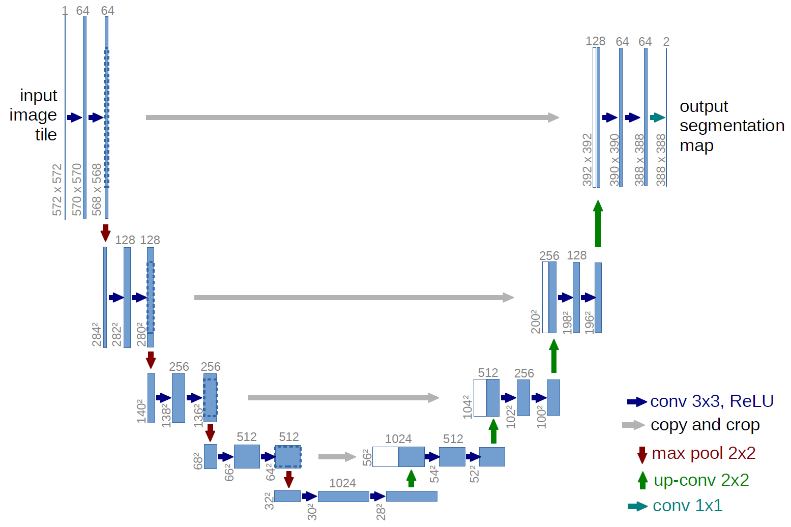 .
. - Here is a link to the University website where they talk about the U-Net. But basically this bit down on the left hand side is what a normal convolutional neural network looks like. It’s something which starts with a big image and gradually makes it smaller and smaller until eventually you just have one prediction. What a U-Net does is it then takes that and makes it bigger and bigger and bigger again, and then it takes every stage of the downward path and copies it across, and it creates this U shape.
- It is a bit like a convolutional autoencoder except there are these data sharing links that cross horizontal across the network in the diagram.
- In fastai you create a UNET with
unet_learner(data, models.resnet34, metrics=metrics, wd=wd)and you pass in all the same stuff as withcnn_learner.
Results
With UNET and the default fastai results Jeremy managed to achieve a SOTA result of 0.92 accuracy.
BIWI Head Pose: Regression
(Link to Notebook)

In this problem we want to locate the center point of the face of a person in an image.
So far, everything we’ve done has been a classification model﹣something that created labels or classes. This, for the first time, is what we call a regression model. A lot of people think regression means linear regression, it doesn’t. Regression just means any kind of model where your output is some continuous number or set of numbers. So we need to create an image regression model (i.e. something that can predict these two numbers). How do you do that? Same way as always - data bunch api then CNN model.
Loading the Data
tfms = get_transforms(max_rotate=20, max_zoom=1.5, max_lighting=0.5, max_warp=0.4, p_affine=1., p_lighting=1.)

data = (PointsItemList.from_folder(path)
        .split_by_valid_func(lambda o: o.parent.name=='13')
        .label_from_func(get_ctr)
        .transform(tfms, tfm_y=True, size=(120,160))
        .databunch().normalize(imagenet_stats)
       )
This is exactly the same as we have already seen except the target variable is represented as a different data type - the ImagePoints class. An ImagePoints object represents a ‘flow’ (it’s just a list) of 2D points on an image. The points have the convention of (y, x) and are scaled to be between -1 and 1.
An example flow looks like:
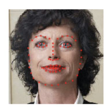
In the case of BIWI, there is only one point in the flow however, but you get the idea. For facial keypoints type problems ImagePoints is what you want to use.
When it comes to training the model you use the same cnn_learner as in the other examples, the only difference being the loss function. For problems where you are predicting a continuous value like here you typically use the Mean Squared Error (MSELossFlat() in fastai) as the loss function. In fastai you don’t need to specify this, cnn_learner will select it for you.
IMDB: Text Classification
(Link to the Notebook)
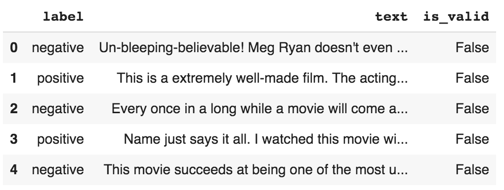
This is a short section on a Natural Language Processing (NLP) problem. Instead of classifying images we will look classifying documents. We will use the IMDB data set and classify if a movie review is negative or positive.
Use different fastai module for text:
from fastai.text import *
Loading the Data
The data is a csv and looks like:
Use the datablock/databunch API to load the csv for text data types:
data_lm = TextDataBunch.from_csv(path, 'texts.csv')
From this you can create a learner and train on this. There are two steps not shown here that transform the text from text to something that you can give to a neural network to train on (i.e. numbers). These steps are Tokenization and Numericalization.
Tokenization
Split raw sentences into words, or ‘tokens’. It does this by:
- Splitting the string into just the words
- Takes care of punctuation
- Separates contractions from words: “didn’t” -> “did” + “n’t”
- Replacing unknown words with a single token “xxunk”.
- Cleaning out HTML from the text.
data = TextClasDataBunch.from_csv(path, 'texts.csv', valid_pct=0.01)
data.show_batch()
Example:
“Raising Victor Vargas: A Review
You know, Raising Victor Vargas is like sticking your hands into a big, steaming bowl of oatmeal. It’s warm and gooey, but you’re not sure if it feels right. Try as I might, no matter how warm and gooey Raising Victor Vargas became I was always aware that something didn’t quite feel right. …
=>
xxbos xxmaj raising xxmaj victor xxmaj vargas : a xxmaj review \n \n xxmaj you know , xxmaj raising xxmaj victor xxmaj vargas is like sticking your hands into a big , steaming bowl of xxunk . xxmaj it ‘s warm and gooey , but you ‘re not sure if it feels right . xxmaj try as i might , no matter how warm and gooey xxmaj raising xxmaj …
Anything starting with ‘xx’ is some special token.
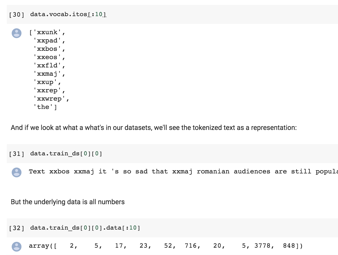
Numericalization
Once we have extracted the tokens from the text, we can convert them to integers by create a big list of all the tokens used: vocabulary. This list only includes words that are used at least twice and is truncated with a maximum size of 60,000 (by default). Words that don’t make the cut are replaced with ‘XXUNK’.
From the notebook:
With the data block API
Here are the previous steps done this time with the data block API:
data = (TextList.from_csv(path, 'texts.csv', cols='text')
                .split_from_df(col=2)
                .label_from_df(cols=0)
                .databunch())
Training a Classifier Preview
Lesson 4 covers the training of the text classifier in detail. Here are the steps covered as a preview.
- You need to first create a language model trained on your text corpus. fastai has
language_model_learnerfor this. This training is quite time/compute intensive. - Then you create a text classifier -
text_classifier_model- and use the language model trained in 1 as the feature encoder.
What is deep learning fundamentally?
Up to this point we’ve seen loads of different problems that deep learning helps us tackle. Deep learning is buzzword for algorithms that use these things called neural networks, which sound like something complicated that may have something to do with how the human brain works. If you remove all the mystique from deep learning you see that it is basically a model with parameters that are updated using Stochastic Gradient Descent. These parameters are parameters to matrix multiplications (convolutions also a tweaked kind of matrix multiplication).
A matrix multiply is a linear function and any stacking of matrix multiplies is a also a linear function because of linearity. Telling the difference between cats and dogs is far more than a linear function can do. So after the matrix multiplications we have something called a non-linearity of activation function. This takes the result of the matrix multiplication and sticks it through some non-linear function.
In the old days the most common function used was the sigmoid, e.g. tanh:

These days the workhorse is the rectified linear unit (ReLU):

Sounds fancy, but in reality it’s this:
def relu(x): max(x, 0)
So how can a stack of matrix multiplications and relu’s result in a model that can classify IMDB reviews or galaxies? Because of a thing called the Universal Approximation Theorem. What it says is that if you have stacks of linear functions and nonlinearities, the thing you end up with can approximate any function arbitrarily closely. So you just need to make sure that you have a big enough matrix to multiply by, or enough of them. If you have this function which is just a sequence of matrix multiplies and nonlinearities where the nonlinearities can be basically any of these activation functions, if that can approximate anything, then all you need is some way to find the particular values of the weight matrices in your matrix multiplies that solve the problem you want to solve. We already know how to find the values of parameters. We can use gradient descent. So that’s actually it.
There is a nice website that has interactive javascript demos that demonstrate this: http://neuralnetworksanddeeplearning.com.
Jeremy Says…
- If you use a dataset, it would be very nice of you to cite the creator and thank them for their dataset.
- This week, see if you can come up with a problem that you would like to solve that is either multi-label classification or image regression or image segmentation or something like that and see if you can solve that problem. Context: Fast.ai Lesson 3 Homework 36
- Always use the same stats that the model was trained with (e.g. imagenet). (See relevant question in Q & A section). Context: Lesson 3: Normalized data and ImageNet 7
Q & A
- When your model makes an incorrect prediction in a deployed app, is there a good way to “record” that error and use that learning to improve the model in a more targeted way? [42:01]
- If you had, for example, an image classifier online you could have a user tell you if the classifier got it wrong and what the right answer is.
- You could then store that image that was incorrectly classified.
- Every so often you could go and fine-tune your network on a new data bunch of just the misclassified images.
- You do this by taking your existing network, unfreezing the layers, and then run some epochs on the misclassified images. You may want to run with a slightly higher learning rate or for more epochs because these images are more interesting/suprising to the model.
-
What resources do you recommend for getting started with video? For example, being able to pull frames and submit them to your model. [47:39]
The answer is it depends. If you’re using the web which I guess probably most of you will be then there’s web API’s that basically do that for you. So you can grab the frames with the web API and then they’re just images which you can pass along. If you’re doing a client side, I guess most people would tend to use OpenCV for that. But maybe during the week, people who are doing these video apps can tell us what have you used and found useful, and we can start to prepare something in the lesson wiki with a list of video resources since it sounds like some people are interested.
-
Is there a way to use
learn.lr_find()and have it return a suggested number directly rather than having to plot it as a graph and then pick a learning rate by visually inspecting that graph? (And there are a few other questions around more guidance on reading the learning rate finder graph) [1:00:26]The short answer is no and the reason the answer is no is because this is still a bit more artisanal than I would like. As you can see, I’ve been saying how I read this learning rate graph depends a bit on what stage I’m at and what the shape of it is. I guess when you’re just training the head (so before you unfreeze), it pretty much always looks like this:

And you could certainly create something that creates a smooth version of this, finds the sharpest negative slope and picked that. You would probably be fine nearly all the time.
But then for you know these kinds of ones, it requires a certain amount of experimentation:

But the good news is you can experiment. Obviously if the lines going up, you don’t want it. Almost certainly at the very bottom point, you don’t want it right there because you needed to be going downwards. But if you kind of start with somewhere around 10x smaller than that, and then also you could try another 10x smaller than that. Try a few numbers and find out which ones work best.
And within a small number of weeks, you will find that you’re picking the best learning rate most of the time. So at this stage, it still requires a bit of playing around to get a sense of the different kinds of shapes that you see and how to respond to them. Maybe by the time this video comes out, someone will have a pretty reliable auto learning rate finder. We’re not there yet. It’s probably not a massively difficult job to do. It would be an interesting project﹣collect a whole bunch of different datasets, maybe grab all the datasets from our datasets page, try and come up with some simple heuristic, compare it to all the different lessons I’ve shown. It would be a really fun project to do. But at the moment, we don’t have that. I’m sure it’s possible but we haven’t got them.
-
Could you use unsupervised learning here (pixel classification with the bike example) to avoid needing a human to label a heap of images[1:10:03]
Not exactly unsupervised learning, but you can certainly get a sense of where things are without needing these kind of labels. Time permitting, we’ll try and see some examples of how to do that. You’re certainly not going to get as such a quality and such a specific output as what you see here though. If you want to get this level of segmentation mask, you need a pretty good segmentation mask ground truth to work with.
-
Is there a reason we shouldn’t deliberately make a lot of smaller datasets to step up from in tuning? let’s say 64x64, 128x128, 256x256, etc… [1:10:51]
Yes, you should totally do that. It works great. This idea, it’s something that I first came up with in the course a couple of years ago and I thought it seemed obvious and just presented it as a good idea, then I later discovered that nobody had really published this before. And then we started experimenting with it. And it was basically the main tricks that we use to win the DAWNBench ImageNet training competition.
Not only was this not standard, but nobody had heard of it before. There’s been now a few papers that use this trick for various specific purposes but it’s still largely unknown. It means that you can train much faster, it generalizes better. There’s still a lot of unknowns about exactly how small, how big, and how much at each level and so forth. We call it “progressive resizing”. I found that going much under 64 by 64 tends not to help very much. But yeah, it’s a great technique and I definitely try a few different sizes.
-
What does accuracy mean for pixel wise segmentation? Is it
#correctly classified pixels / #total number of pixels? [1:12:35]Yep, that’s it. So if you imagined each pixel was a separate object you’re classifying, it’s exactly the same accuracy. So you actually can just pass in
accuracyas your metric, but in this case, we actually don’t. We’ve created a new metric calledacc_camvidand the reason for that is that when they labeled the images, sometimes they labeled a pixel asVoid. I’m not quite sure why but some of the pixels areVoid. And in the CamVid paper, they say when you’re reporting accuracy, you should remove the void pixels. So we’ve created accuracy CamVid. So all metrics take the actual output of the neural net (i.e. that’s theinputto the metric) and the target (i.e. the labels we are trying to predict).
We then basically create a mask (we look for the places where the target is not equal to
Void) and then we just take the input, do theargmaxas per usual, but then we just grab those that are not equal to the void code. We do the same for the target and we take the mean, so it’s just a standard accuracy.It’s almost exactly the same as the accuracy source code we saw before with the addition of this mask. This quite often happens. The particular Kaggle competition metric you’re using or the particular way your organization scores things, there’s often little tweaks you have to do. And this is how easy it is. As you’ll see, to do this stuff, the main thing you need to know pretty well is how to do basic mathematical operations in PyTorch so that’s just something you kind of need to practice.
-
I’ve noticed that most of the examples and most of my models result in a training loss greater than the validation loss. What are the best ways to correct that? I should add that this still happens after trying many variations on number of epochs and learning rate. [1:15:03]
Remember from last week, if your training loss is higher than your validation loss then you’re underfitting. It definitely means that you’re underfitting. You want your training loss to be lower than your validation loss. If you’re underfitting, you can:
- Train for longer.
- Train the last bit at a lower learning rate.
But if you’re still under fitting, then you’re going to have to decrease regularization. We haven’t talked about that yet. In the second half of this part of the course, we’re going to be talking quite a lot about regularization and specifically how to avoid overfitting or underfitting by using regularization. If you want to skip ahead, we’re going to be learning about:
- weight decay
- dropout
- data augmentation
They will be the key things that are we talking about.
-
For a dataset very different than ImageNet like the satellite images or genomic images shown in lesson 2, we should use our own stats. Jeremy once said: “If you’re using a pretrained model you need to use the same stats it was trained with.” Why it is that? Isn’t it that, normalized dataset with its own stats will have roughly the same distribution like ImageNet? The only thing I can think of, which may differ is skewness. Is it the possibility of skewness or something else the reason of your statement? And does that mean you don’t recommend using pre-trained model with very different dataset like the one-point mutation that you showed us in lesson 2? [1:46:53]
Nope. As you can see, I’ve used pre-trained models for all of those things. Every time I’ve used an ImageNet pre-trained model, I’ve used ImageNet stats. Why is that? Because that model was trained with those stats. For example, imagine you’re trying to classify different types of green frogs. If you were to use your own per-channel means from your dataset, you would end up converting them to a mean of zero, a standard deviation of one for each of your red, green, and blue channels. Which means they don’t look like green frogs anymore. They now look like grey frogs. But ImageNet expects frogs to be green. So you need to normalize with the same stats that the ImageNet training people normalized with. Otherwise the unique characteristics of your dataset won’t appear anymore﹣you’ve actually normalized them out in terms of the per-channel statistics. So you should always use the same stats that the model was trained with.
-
There’s a question about tokenization. I’m curious about how tokenizing words works when they depend on each other such as San Francisco. [1:56:45]
How do you tokenize something like San Francisco. San Francisco contains two tokens
SanFrancisco. That’s it. That’s how you tokenize San Francisco. The question may be coming from people who have done traditional NLP which often need to use these things called n-grams. N-rams are this idea of a lot of NLP in the old days was all built on top of linear models where you basically counted how many times particular strings of text appeared like the phrase San Francisco. That would be a bi-gram for an n-gram with an n of 2. The cool thing is that with deep learning, we don’t have to worry about that. Like with many things, a lot of the complex feature engineering disappears when you do deep learning. So with deep learning, each token is literally just a word (or in the case that the word really consists of two words likeyou'reyou split it into two words) and then what we’re going to do is we’re going to then let the deep learning model figure out how best to combine words together. Now when we see like let the deep learning model figure it out, of course all we really mean is find the weight matrices using gradient descent that gives the right answer. There’s not really much more to it than that.Again, there’s some minor tweaks. In the second half of the course, we’re going to be learning about the particular tweak for image models which is using a convolution that’ll be a CNN, for language there’s a particular tweak we do called using recurrent models or an RNN, but they’re very minor tweaks on what we’ve just described. So basically it turns out with an RNN, that it can learn that
SanplusFranciscohas a different meaning when those two things are together. -
Some satellite images have 4 channels. How can we deal with data that has 4 channels or 2 channels when using pre-trained models? [1:59:09]
I think that’s something that we’re going to try and incorporate into fast AI. So hopefully, by the time you watch this video, there’ll be easier ways to do this. But the basic idea is a pre-trained ImageNet model expects a red green and blue pixels. So if you’ve only got two channels, there’s a few things you can do but basically you’ll want to create a third channel. You can create the third channel as either being all zeros, or it could be the average of the other two channels. So you can just use you know normal PyTorch arithmetic to create that third channel. You could either do that ahead of time in a little loop and save your three channel versions, or you could create a custom dataset class that does that on demand.
For 4 channel, you probably don’t want to get rid of the 4th channel. So instead, what you’d have to do is to actually modify the model itself. So to know how to do that, we’ll only know how to do in a couple more lessons time. But basically the idea is that the initial weight matrix (weight matrix is really the wrong term, they’re not weight matrices; their weight tensors so they can have more than just two dimensions), so that initial weight tensor in the neural net, one of its axes is going to have three slices in it. So you would just have to change that to add an extra slice, which I would generally just initialize to zero or to some random numbers. So that’s the short version. But really to understand exactly what I meant by that, we’re going to need a couple more lessons to get there.
Links and References
- Lesson video: https://course.fast.ai/videos/?lesson=3
- Homework notebooks:
- Notebook 1: lesson3-planet.ipynb
- Notebook 2: lesson3-camvid.ipynb
- Notebook 3: lesson3-imdb.ipynb
- Notebook 4: lesson3-head-pose.ipynb
- Parts of my notes have been copied from the excellent lecture transcriptions made by @hiromi. Link: Lesson3 Detailed Notes.
- Universal approximation theorem + more: http://neuralnetworksanddeeplearning.com
- Source for Jeremy says: https://forums.fast.ai/t/things-jeremy-says-to-do/36682
- Cyclical Learning Rates for Training Neural Networks paper by Leslie Smith