
Overview of Lesson
This is the introductory lesson to fastai part 1!
The key outcome of this lesson is that we’ll have trained an image classifier which can recognize pet breeds at state of the art accuracy. The key to this success is the use of transfer learning, which will be a key platform for much of this course. We’ll also see how to analyze the model to understand its failure modes. In this case, we’ll see that the places where the model is making mistakes is in the same areas that even breeding experts can make mistakes.
Task 1 - World Class Image Classifier
-
Fastai opts to teach deep learning backwards - rather than starting at the level of neurons they start with learning to use the state of the art algorithms and networks from the beginning. Learning to become a practitioner with the best practices first and then gradually learning the technical details later.
-
Task 1: Training a world class image classification model.
-
Image classification has been one of deep learning’s biggest successes so far.
-
10 years ago separating cat and dog images was a hard problem. With classical methods researchers were scoring ~80%. With today’s algorithms it’s actually too easy and scores on the cats vs dogs dataset are almost 100%. That’s why we used the harder dataset of cat and dog breeds.
-
Cat breeds and dog breeds dataset from Oxford: Cats and Dogs Breeds Classification Oxford Dataset | Kaggle.
-
This task found in the Jupyter notebook: lesson1-pets.pynb
Load the Data
-
FastAI has its own way of handling different datasets: the DataBunch API.
-
This integrates the loading of different types of data, the labeling, splitting into train/val/test, and the data transformations for standardisation, normalisation, and training augmentation.
-
To load the cats and dogs dataset:
pat = r'/([^/]+)_\d+.jpg$' data = ImageDataBunch.from_name_re(path_img, fnames, pat, ds_tfms=get_transforms(), size=224, bs=64, ).normalize(imagenet_stats) -
What is this doing? Let’s look at the docs:
class ImageDataBunch(fastai.basic_data.DataBunch) | DataBunch suitable for computer vision. ... | from_name_re(path:Union[pathlib.Path, str], fnames:Collection[pathlib.Path], pat:str, valid_pct:float=0.2, **kwargs) from builtins.type | Create from list of `fnames` in `path` with re expression `pat`. get_transformsis a function that returns a list of default image transformations for data augmentation.size=224resizes the images to224x224. This is the size that the network we are using (resnet34) has been trained on.bsis the batchsize.normalize(imagenet_stats)normalizes the images so that the pixel values are between 0 and 1 (necessary for using the neural network). The network has been pretrained on imagenet data so we need to normalize our new data with respect to the imagenet data. This way the images are placed near the distribution that the network was trained on and so gives the network data that it is ‘used to’ seeing.
Training a Model using a Pretrained ResNet
-
‘ResNet’ is the name of a particular kind of Convolutional Neural Network (CNN). Details of it will be covered later.
-
The ResNet we will use has been pretrained. This means that it was trained to solve another image classification problem (namely ImageNet) and we are reusing the learned weights of that network as a starting point for a new imaging problem.
-
Why ResNet and not some other architecture? From looking at benchmarks it has been found that ResNet generally ‘just works well’ for image tasks. (See also question in Q & A section below).
-
Here’s how to create a CNN with the fastai library:
learn = create_cnn(data, models.resnet34, metrics=error_rate) -
datais the DataBunch object of the cats/dogs data we created earlier. -
Here we are using a variant of ResNet called
resnet34. The 34 simply means it has 34 layers. There are others avaiable with 18, 50, and more layers. -
One-cycle policy:
-
learn.fit_one_cycle(4) -
People train neural networks using Stochastic Gradient Descent (SGD). Here the training set is divided into random batches (say of size 64) and the network weights are updated after each batch. After the network has seen all the batches, this is called an epoch. The rate at which the weights are changed is called the learning rate. Typically people set this to a single value that remains unchanged during an epoch. Not here though.
-
The One-cycle policy is a way of training the neural network using SGD faster by varying the learning rate and solver momentum over a group of epochs.
-
Sylvain explains (source):
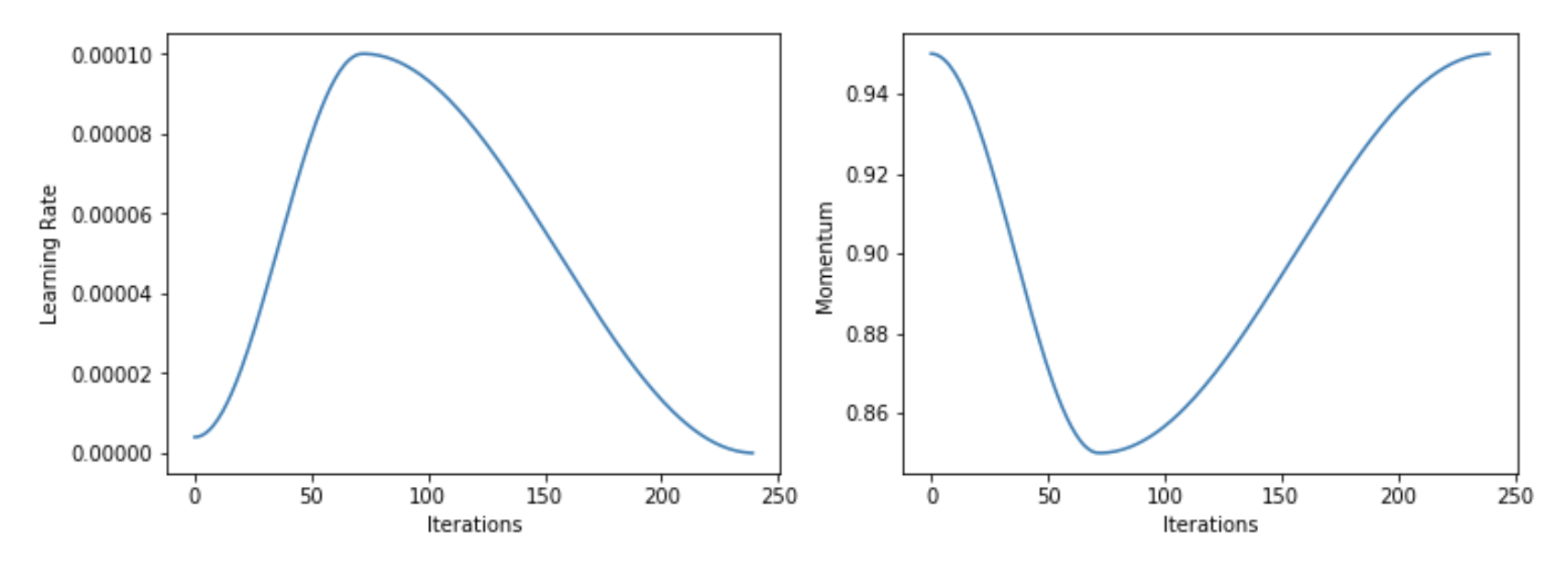
He [Leslie] recommends to do a cycle with two steps of equal lengths, one going from a lower learning rate to a higher one than go back to the minimum. The maximum should be the value picked with the Learning Rate Finder, and the lower one can be ten times lower. Then, the length of this cycle should be slightly less than the total number of epochs, and, in the last part of training, we should allow the learning rate to decrease more than the minimum, by several orders of magnitude.
-
Here are plots of how the learning rate and momentum vary over the iterations (batches):
-
The peak of the learning rate has a value of 1x the inputted learning rate. The bottom value is 0.1x the inputted learning rate. The bottom of the momentum value is 0.85x the inputted momentum value.
-
The momentum varies contra to the learning rate. What’s the intuition behind this? When the learning rate is high we want momentum to be lower. This enables the SGD to quickly change directions and find a flatter region in parameter space.
-
-
Learning Rate Finder
-
The method is basically successively increasing $\eta$ every batch using either a linear or exponential schedule and looking the loss. While $\eta$ has a good value, the loss will be decreasing. When $\eta$ gets too large the loss will start to increase. You can plot the loss versus $\eta$ and see by eye a learning rate that is largest where the loss is decreasing fastest.
-
learn.lr_find() learn.recorder.plot() -

- More on this will be covered in the next lesson.
-
Getting Started With the Notebooks
-
All the course notebooks for part 1 are found here: [notebooks github](https://github.com/fastai/course-v3/tree/master/nbs/dl1). - The course guide can be found here: course guide.
- For running and experimenting with the fastai notebooks I personally like to use:
Jeremy Says…
- Don’t try to stop and understand everything.
- Don’t waste your time, learn Jupyter keyboard shortcuts. Learn 4 to 5 each day.
- Please run the code, really run the code. Don’t go deep on theory. Play with the code, see what goes in and what comes out.
- Pick one project. Do it really well. Make it fantastic.
- Run this notebook (lesson1-pets.ipynb), but then get your own dataset and run it! (extra emphasis: do this!) If you have a lot of categories, don’t run confusion matrix, run…
interp.most_confused(min_val=n)
Q & A
-
As GPU mem will be in power of 2, doesn’t size 256 sound more practical considering GPU utilization compared to 224?
The brief answer is that the models are designed so that the final layer is of size 7 by 7, so we actually want something where if you go 7 times 2 a bunch of times (224 = 7x2x2x2x2x2), then you end up with something that’s a good size. Objects often appear in the middle of an image in the ImageNet dataset. After 5 maxpools, a 224x224 will be 7x7 meaning that it will have a centerpoint. A 256x256 image will be 8x8 and not have a distinct centerpoint.
-
Why resnet and not inception architecture?
Resnet is Good Enough! See the DAWN benchmarks - the top 4 are all Resnet.You can consider different models for different use cases. For example, if you want to do edge computing, mobile apps, Jeremy still suggests running the model on the local server and port results to the mobile device. But if you want to run something on the low powered device, there are special architectures for that.
Inception is pretty memory intensive. fastai wants to show you ways to run your model without much fine-tuning and still achieve good results. The kind of stuff that always tends to work. Resnet works well on a lot of image classification applications.
-
Will the library use multi GPUs in parallel by default?
The library will use multiple CPUs by default but just one GPU by default. We probably won’t be looking at multi GPU until part 2. It’s easy to do and you’ll find it on the forum, but most people won’t be needing to use that now.
Links and References
- Link to Lesson 1 lecture
- Homework notebooks:
- Notebook 1: lesson1-pets.pynb
- Detailed lesson notes - thanks to @hiromi
- Stanford DAWN Deep Learning Benchmark (DAWNBench) ·
- [1311.2901] Visualizing and Understanding Convolutional Networks
- Another data science student’s blog – The 1cycle policy
- Learning Rate Finder Paper