
Overview of the Lesson
This lesson looks at the fundament components of deep learning - parameters, activations, backpropagation, transfer learning, and discriminative learning rates.
Components of Deep Learning
Roughly speaking, this is the bunch of concepts that we need to learn about -
- Inputs
- Weights/parameters
- Random
- Activations
- Activation functions / nonlinearities
- Output
- Loss
- Metric
- Cross-entropy
- Softmax
- Fine tuning
- Layer deletion and random weights
- Freezing & unfreezing
Diagram of a neural network:
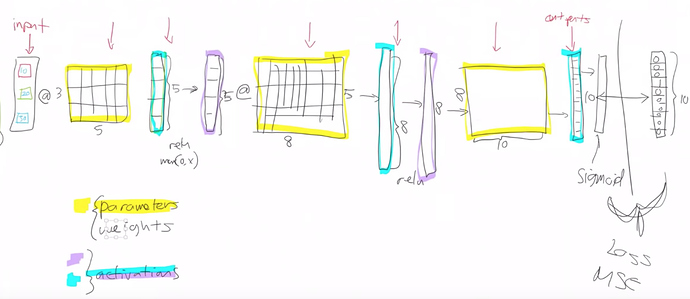
There are three types of layer in a NN:
-
Input.
-
Weights/Parameters: These are layers that contain parameters or weights. These are things like matrices or convolutions. Parameters are used by multiplying them by input activations doing a matrix product. The yellow things in the above diagram are our weight matrices / weight tensors. Parameters are the things that your model learns in train via gradient descent:
weights = weights - learning_rate * weights.grad -
Activations: These are layers that contain activations, also called as non-linear layers which are stateless. For example, ReLu, softmax, or sigmoid.
Here is the process of input, weight multiplication, and activation up close (image credit):
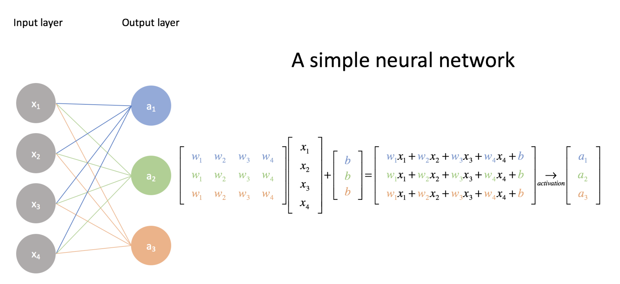
The parameters/weights are the matrix $\mathbf{W}$, the input is the vector $x$, and there is also the bias vector $b$. This can be expressed mathematically as: \(\mathbf{a} = g(\mathbf{W^T}\mathbf{x} + \mathbf{b})\) Let’s get an intuition for how the dimension of the data changes as it flows through the network. In the diagram above there is an input vector of size 4 and a weight matrix of size 4x3. The matrix vector product in terms of just the dimensions is: $(4, 3)^T \cdot (4) = (3, 4) \cdot (4) = (3)$.
In summation notation this is $(W_{ji})^Tx_j = W_{ij} x_j = a_i$. The $j$ terms are summed out and we are left with $i$ dimension only.
The activation function is an element-wise function. It’s a function that is applied to each element of the input, activations in turn and creates one activation for each input element. If it starts with a twenty long vector it creates a twenty long vector by looking at each one of those, in turn, doing one thing to it and spitting out the answer, so an element-wise function. These days the activation function most often used is ReLu.
Backpropagation
After the loss has been calculated from the different between the output and the ground truth, how are millions of parameters in the network then updated? This is done by a clever algorithm called backpropogation. This algorithm calculates the partial derivatives of the loss with respect to every parameter in the network. It does this using the chain-rule from calculus. The best explanation of this I’ve seen is from Chris Olah’s blog.
In PyTorch, these derivatives are calculated automatically for you (aka autograd) and the gradient of any PyTorch variable is stored in its .grad attribute.
Mathematically the weights are updated like so: \(w_t = w_{t-1} - lr \times \frac{\partial L}{\partial w_{t-1}}\)
How is Transfer Learning Done?
What happens when we take a resnet34 trained on ImageNet and we do transfer learning? How can a network that is trained to identify 1000 different everyday objects be repurposed for, say, identifying galaxies?
Let’s look at some examples we’ve seen already. Here are is the last layer group of the resnet34 used in the dog/cat breed example:
  (1): Sequential(
    (0): AdaptiveConcatPool2d(
      (ap): AdaptiveAvgPool2d(output_size=1)
      (mp): AdaptiveMaxPool2d(output_size=1)
    )
    (1): Flatten()
    (2): BatchNorm1d(1024, eps=1e-05, momentum=0.1, affine=True, track_running_stats=True)
    (3): Dropout(p=0.25)
    (4): Linear(in_features=1024, out_features=512, bias=True)
    (5): ReLU(inplace)
    (6): BatchNorm1d(512, eps=1e-05, momentum=0.1, affine=True, track_running_stats=True)
    (7): Dropout(p=0.5)
    (8): Linear(in_features=512, out_features=37, bias=True)
  )
And here is the same layer group from the head pose example:
  (1): Sequential(
    (0): AdaptiveConcatPool2d(
      (ap): AdaptiveAvgPool2d(output_size=1)
      (mp): AdaptiveMaxPool2d(output_size=1)
    )
    (1): Flatten()
    (2): BatchNorm1d(1024, eps=1e-05, momentum=0.1, affine=True, track_running_stats=True)
    (3): Dropout(p=0.25)
    (4): Linear(in_features=1024, out_features=512, bias=True)
    (5): ReLU(inplace)
    (6): BatchNorm1d(512, eps=1e-05, momentum=0.1, affine=True, track_running_stats=True)
    (7): Dropout(p=0.5)
    (8): Linear(in_features=512, out_features=2, bias=True)
  )
The two layers that change here are (4) and (8).
- Layer (4) is a matrix with some default size that is the same in both cases. It anyway needs to be relearned for a new problem.
- Layer (8) is different in
out_features. This is the dimensionality of the output. There are 37 cat/dog breeds in the first example, and there are x and y coordinates in the second. Layer (8) is a Linear layer – i.e. it’s a matrix!
So to do transfer learning we just need to swap out the last matrix with a new one.
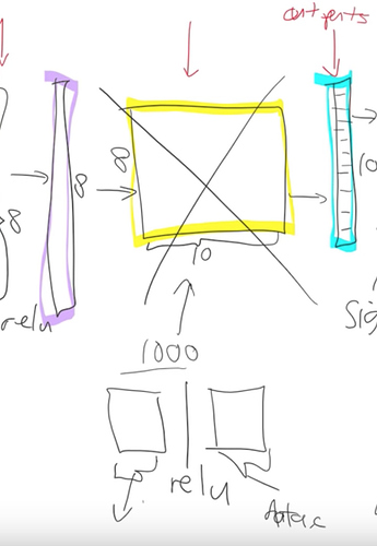
For an imagenet network this matrix would have shape (512, 1000), for the cat/dog (512, 37), and for the head pose (512, 2). Every row in this matrix represents a category you are predicting.
Fastai library figures out the right size for this matrix by looking at the data bunch you passed to it.
Freezing Layers
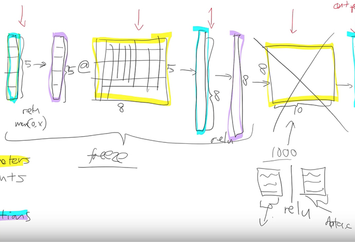
The new head of the network has two randomly initialized matrices. They need to be trained because they are random, however the rest of the network is quite well trained on imagenet already - they are vastly better than random even though they weren’t trained on the task at hand.
So we freeze all the layers before the head, which means we don’t update their parameters during training. It’ll be a little bit faster because there are fewer calculations to do, and also it will save some memory because there are fewer gradients to store.
After training a few epochs with just the head unfrozen, we are ready to train the whole network. So we unfreeze everything.
Discriminative Learning Rates
Now we’re going to train the whole thing but we still have a pretty good sense that these new layers we added to the end probably need more training and these ones right at the start that might just be like diagonal edges probably don’t need much training at all.
Let’s review what the different layers in a CNN learn to do first. The first layer visualized looks like this:
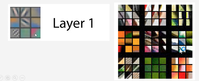
This layer is good at finding diagonal lines in different directions.
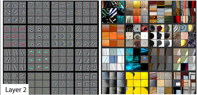
In layer 2 some of the filters were good at spotting corners in the bottom right corner.
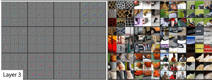
In layer 3, one of the filters found repeating patterns or round orange things or fluffy or floral textures.
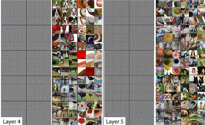
As we go deeper, they’re becoming more sophisticated but also more specific. By layer 5, It could find bird eyeballs or dog faces.
If you’re wanting to transfer and learn to something for galaxy morphology there’s probably going to be no eyeballs in that dataset. So the later layers are no good to you but there will certainly be some repeating patterns or some diagonal edges. The earlier a layers is in the pretrained model the more likely it is that you want those weights to stay as they are.
We can implement this by splitting the model into a few sections and giving the earlier sections slower learning rates. Earlier layers of the model we might give a learning rate of 1e - 5 and newly added layers of the model we might give a learning rate of 1e - 3. What’s gonna happen now is that we can keep training the entire network. But because the learning rate for the early layers is smaller it’s going to move them around less because we think they’re already pretty good. If it’s already pretty good to the optimal value if you used a higher learning rate it could kick it out. It could actually make it worse which we really don’t want to happen.
In fastai this is done with any of the following lines of code:
learn.fit_one_cycle(5, 1e-3)
learn.fit_one_cycle(5, slice(1e-3))
learn.fit_one_cycle(5, slice(1e-5, 1e-3))
These mean:
- A single number like
1e-3: Just using a single number means every layer gets the same learning rate so you’re not using discriminative learning rates. - A slice with a single number
slice(1e-3):If you pass a single number to slice it means the final layers get a learning rate of1e-3and then all the other layers get the same learning rate which is that divided by 3. All of the other layers will be(1e-3)/3and the last layers will be1e-3. - A slice with two numbers,
slice(1e-5, 1e-3)In the last case, the final layers the these randomly hidden added layers will still be again1e-3. The first layers will get1e-5. The other layers will get learning rates that are equally spread between those two. Multiplicatively equal. If there were three layers there would be1e-5,1e-4and1e-3. Multiplied by the same factor between layers each time.
This divided by 3 thing that is a little weird and we won’t talk about why that is until part two of the course. it is specific quirk around batch normalization.
Collaborative Filtering: Deep Dive
Recall from the previous lesson the movie recommendation problem.
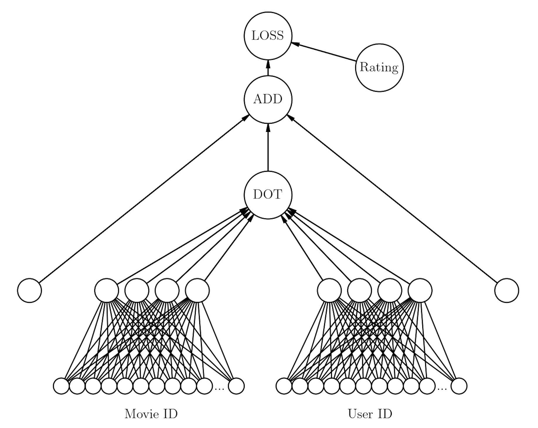
For the movielens dataset the model looks like:
$> learn.model

  EmbeddingDotBias(
    (u_weight): Embedding(944, 40)
    (i_weight): Embedding(1654, 40)
    (u_bias): Embedding(944, 1)
    (i_bias): Embedding(1654, 1)
  )
We already know what u_weight and i_weight are: the user and movie embedding matrices, respectively. What are the additional components of the model: u_bias and i_bias?
Interpreting Bias
These are the 1D bias terms for the movies and films. In the model diagram above these are the two edge nodes on the left and right that connect to the ADD node.
Every user and every movie has its own bias term.
-
You can interpret user bias as how much that user likes movies.
-
You can interpret movie bias as how well liked a movie is in general. (Ironically, the bias is the unbiased movie score).
Here are the movies with the highest bias alongside their actual movie rating:
movie_bias = learn.bias(top_movies, is_item=True)
Top 10:
[(tensor(0.6105), "Schindler's List (1993)", 4.466442953020135),
 (tensor(0.5817), 'Titanic (1997)', 4.2457142857142856),
 (tensor(0.5685), 'Shawshank Redemption, The (1994)', 4.445229681978798),
 (tensor(0.5451), 'L.A. Confidential (1997)', 4.161616161616162),
 (tensor(0.5350), 'Rear Window (1954)', 4.3875598086124405),
 (tensor(0.5341), 'Silence of the Lambs, The (1991)', 4.28974358974359),
 (tensor(0.5330), 'Star Wars (1977)', 4.3584905660377355),
 (tensor(0.5227), 'Good Will Hunting (1997)', 4.262626262626263),
 (tensor(0.5114), 'As Good As It Gets (1997)', 4.196428571428571),
 (tensor(0.4800), 'Casablanca (1942)', 4.45679012345679),
 (tensor(0.4698), 'Boot, Das (1981)', 4.203980099502488),
 (tensor(0.4589), 'Close Shave, A (1995)', 4.491071428571429),
 (tensor(0.4567), 'Apt Pupil (1998)', 4.1),
 (tensor(0.4566), 'Vertigo (1958)', 4.251396648044692),
 (tensor(0.4542), 'Godfather, The (1972)', 4.283292978208232)]
Bottom 10:
[(tensor(-0.4076),
  'Children of the Corn: The Gathering (1996)',
  1.3157894736842106),
 (tensor(-0.3053),
  'Lawnmower Man 2: Beyond Cyberspace (1996)',
  1.7142857142857142),
 (tensor(-0.2892), 'Cable Guy, The (1996)', 2.339622641509434),
 (tensor(-0.2856), 'Mortal Kombat: Annihilation (1997)', 1.9534883720930232),
 (tensor(-0.2530), 'Striptease (1996)', 2.2388059701492535),
 (tensor(-0.2405), 'Free Willy 3: The Rescue (1997)', 1.7407407407407407),
 (tensor(-0.2361), 'Showgirls (1995)', 1.9565217391304348),
 (tensor(-0.2332), 'Bio-Dome (1996)', 1.903225806451613),
 (tensor(-0.2279), 'Crow: City of Angels, The (1996)', 1.9487179487179487),
 (tensor(-0.2273), 'Barb Wire (1996)', 1.9333333333333333),
 (tensor(-0.2246), "McHale's Navy (1997)", 2.1884057971014492),
 (tensor(-0.2197), 'Beverly Hills Ninja (1997)', 2.3125),
 (tensor(-0.2178), "Joe's Apartment (1996)", 2.2444444444444445),
 (tensor(-0.2080), 'Island of Dr. Moreau, The (1996)', 2.1578947368421053),
 (tensor(-0.2064), 'Tales from the Hood (1995)', 2.037037037037037)]
Having seen many of the films in both these lists, I’m not not surprise by what I see here!
Interpreting Weights (the Embeddings)
Grab the weights:
$> movie_w = learn.weight(top_movies, is_item=True)
$> movie_w.shape

	torch.Size([1000, 40])
There are 40 factors in the model. Looking at the 40 latent factors isn’t intuitive or necessarily meaningful so it’s better to squish the 40 factors down to 3 - using Principle Component Analysis (PCA).
$> movie_pca = movie_w.pca(3)
$> movie_pca.shape

	torch.Size([1000, 3])
We can now rank each of the films along these 3 dimensions, knowing film, interpret what these dimensions mean.
Factor 0
fac0,fac1,fac2 = movie_pca.t()
movie_comp = [(f, i) for f,i in zip(fac0, top_movies)]
Top 10:
[(tensor(1.1000), 'Wrong Trousers, The (1993)'),
 (tensor(1.0800), 'Close Shave, A (1995)'),
 (tensor(1.0705), 'Casablanca (1942)'),
 (tensor(1.0304), 'Lawrence of Arabia (1962)'),
 (tensor(0.9957), 'Citizen Kane (1941)'),
 (tensor(0.9792), 'Some Folks Call It a Sling Blade (1993)'),
 (tensor(0.9778), 'Persuasion (1995)'),
 (tensor(0.9752), 'North by Northwest (1959)'),
 (tensor(0.9706), 'Wallace & Gromit: The Best of Aardman Animation (1996)'),
 (tensor(0.9703), 'Chinatown (1974)')]
Bottom 10:
[(tensor(-1.2963), 'Home Alone 3 (1997)'),
 (tensor(-1.2210), "McHale's Navy (1997)"),
 (tensor(-1.2199), 'Leave It to Beaver (1997)'),
 (tensor(-1.1918), 'Jungle2Jungle (1997)'),
 (tensor(-1.1209), 'D3: The Mighty Ducks (1996)'),
 (tensor(-1.0980), 'Free Willy 3: The Rescue (1997)'),
 (tensor(-1.0890), 'Children of the Corn: The Gathering (1996)'),
 (tensor(-1.0873), 'Bio-Dome (1996)'),
 (tensor(-1.0436), 'Mortal Kombat: Annihilation (1997)'),
 (tensor(-1.0409), 'Grease 2 (1982)')]
Interpretation: This dimension is best described as ‘connoisseur movies’.
Factor 1
Top 10:
[(tensor(1.1052), 'Braveheart (1995)'),
 (tensor(1.0759), 'Titanic (1997)'),
 (tensor(1.0202), 'Raiders of the Lost Ark (1981)'),
 (tensor(0.9324), 'Forrest Gump (1994)'),
 (tensor(0.8627), 'Lion King, The (1994)'),
 (tensor(0.8600), "It's a Wonderful Life (1946)"),
 (tensor(0.8306), 'Pretty Woman (1990)'),
 (tensor(0.8271), 'Return of the Jedi (1983)'),
 (tensor(0.8211), "Mr. Holland's Opus (1995)"),
 (tensor(0.8205), 'Field of Dreams (1989)')]
Bottom 10:
[(tensor(-0.8085), 'Nosferatu (Nosferatu, eine Symphonie des Grauens) (1922)'),
 (tensor(-0.8007), 'Brazil (1985)'),
 (tensor(-0.7866), 'Trainspotting (1996)'),
 (tensor(-0.7703), 'Ready to Wear (Pret-A-Porter) (1994)'),
 (tensor(-0.7173), 'Beavis and Butt-head Do America (1996)'),
 (tensor(-0.7150), 'Serial Mom (1994)'),
 (tensor(-0.7144), 'Exotica (1994)'),
 (tensor(-0.7129), 'Lost Highway (1997)'),
 (tensor(-0.7094), 'Keys to Tulsa (1997)'),
 (tensor(-0.7083), 'Jude (1996)')]
Interpretation: This dimension I think can be best described as ‘blockbuster’, or ‘family’.
Factor 2
Top 10:
[(tensor(1.0152), 'Beavis and Butt-head Do America (1996)'),
 (tensor(0.8703), 'Reservoir Dogs (1992)'),
 (tensor(0.8640), 'Pulp Fiction (1994)'),
 (tensor(0.8582), 'Terminator, The (1984)'),
 (tensor(0.8572), 'Scream (1996)'),
 (tensor(0.8058), 'Terminator 2: Judgment Day (1991)'),
 (tensor(0.7728), 'Seven (Se7en) (1995)'),
 (tensor(0.7457), 'Starship Troopers (1997)'),
 (tensor(0.7243), 'Clerks (1994)'),
 (tensor(0.7227), 'Die Hard (1988)')]
Bottom 10:
[(tensor(-0.6912), 'Lone Star (1996)'),
 (tensor(-0.6720), 'Jane Eyre (1996)'),
 (tensor(-0.6613), 'Steel (1997)'),
 (tensor(-0.6227), 'Piano, The (1993)'),
 (tensor(-0.6183), 'My Fair Lady (1964)'),
 (tensor(-0.5946), 'Evita (1996)'),
 (tensor(-0.5827), 'Home for the Holidays (1995)'),
 (tensor(-0.5669), 'Cinema Paradiso (1988)'),
 (tensor(-0.5668), 'All About Eve (1950)'),
 (tensor(-0.5586), 'Sound of Music, The (1965)')]
Regularization: Weight Decay

On the left the model isn’t complex enough. One the right the model has more parameters and is too complex. The middle model has just the right level of complexity.
In Jeremy’s opinion, to reduce model complexity:
- In statistics: they reduce the number of parameters. Jeremy thinks this is wrong.
- In machine learning: they increase the number of parameters, but increase the amount of regularization.
The regularization used in fastai is weight decay (aka L2 regularization). This is where the loss function is modified with an extra component that penalizes extreme values of the weights.
- Unregularized loss:
- L2 regularized loss:
The weight decay parameter $\lambda$ corresponds to the fastai parameter to the Learner model: wd . This is set by default to 0.01.
-
Higher values of
wdgive more regularlization. Looking at the diagram of line fits above, more regularlization makes the line ‘stiffer’ - harder to force through every point. -
Lower values of
wd, conversely, make the line ‘slacker’ - it’s easier to force it through every point. -
It’s worth experimenting with
wdif your model is overfitting or underfitting.
With weight decay the update formula for the weights in gradient descent becomes:
\[w_t = w_{t-1} - lr \times \frac{\partial L}{\partial w_{t-1}} - lr\times \lambda w_{t-1}\](Source)
Jeremy Says…
- The answer to the question “Should I try blah?” is to try blah and see, that’s how you become a good practitioner. Lesson 5: Should I try blah?
- If you want to play around, try to create your own nn.linear class. You could create something called My_Linear and it will take you, depending on your PyTorch experience, an hour or two. We don’t want any of this to be magic and you know everything necessary to create this now. These are the things you should be doing for assignments this week, not so much new applications but trying to write more of these things from scratch and get them to work. Learn how to debug them and check them to see what’s going in and coming out. Lesson 5 Assignment: Create your own version of nn.linear
- A great assignment would be to take Lesson 2 SGD and try to add momentum to it. Or even the new notebook we have for MNIST, get rid of the Optim.SGD and write your own update function with momentum Lesson 5: Another suggested assignment
- It’s definitely worth knowing that taking layers of neural nets and chucking them through PCA is very often a good idea. Because very often you have way more activations than you want in a layer, and there’s all kinds of reasons you would might want to play with it. For example, Francisco who’s sitting next to me today has been working on something to do with image similarity. And for image similarity, a nice way to do that is to compare activations from a model, but often those activations will be huge and therefore your thing could be really slow and unwieldy. So people often, for something like image similarity, will chuck it through a PCA first and that’s kind of cool.
Q & A
-
When we load a pre-trained model, can we explore the activation grids to see what they might be good at recognizing? [36:11]
Yes, you can. And we will learn how to (should be) in the next lesson.
-
Can we have an explanation of what the first argument in
fit_one_cycleactually represents? Is it equivalent to an epoch?Yes, the first argument to
fit_one_cycleorfitis number of epochs. In other words, an epoch is looking at every input once. If you do 10 epochs, you’re looking at every input ten times. So there’s a chance you might start overfitting if you’ve got lots of lots of parameters and a high learning rate. If you only do one epoch, it’s impossible to overfit, and so that’s why it’s kind of useful to remember how many epochs you’re doing. -
What is an affine function?
An affine function is a linear function. I don’t know if we need much more detail than that. If you’re multiplying things together and adding them up, it’s an affine function. I’m not going to bother with the exact mathematical definition, partly because I’m a terrible mathematician and partly because it doesn’t matter. But if you just remember that you’re multiplying things together and then adding them up, that’s the most important thing. It’s linear. And therefore if you put an affine function on top of an affine function, that’s just another affine function. You haven’t won anything at all. That’s a total waste of time. So you need to sandwich it with any kind of non-linearity pretty much works - including replacing the negatives with zeros which we call ReLU. So if you do affine, ReLU, affine, ReLU, affine, ReLU, you have a deep neural network.
-
Why am I sometimes getting negative loss when training? [59:49]
You shouldn’t be. So you’re doing something wrong. Particularly since people are uploading this, I guess other people have seen it too, so put it on the forum. We’re going to be learning about cross entropy and negative log likelihood after the break today. They are loss functions that have very specific expectations about what your input looks like. And if your input doesn’t look like that, then they’re going to give very weird answers, so probably you press the wrong buttons. So don’t do that.
Links and References
- Lesson video: Lesson 5
- Parts of my notes were copied from the excellent lecture transcriptions made by @PoonamV: Lecture notes
- Homework notebooks:
- Notebook 1: SGD and MNIST
- Notebook 2: Rossmann (tabular data)
- Netflix and Chill: Building a Recommendation System in Excel - Latent Factor Visualization in Excel blog post
- An overview of gradient descent optimization algorithms - Sebastian Ruder