
The Fleuron Project
I have been involved in the Fleuron project this year. The aim of this project is to use computer vision to extract printers’ ornaments from a large corpus of ~150,000 scanned documents (32 million pages) from the 18th century. Printed books in the 18th century were highly decorated with miniature pieces of printed artwork - ‘ornaments’. Their pages were adorned with ornaments that ranged from small floral embellishments to large and intricate head- and tailpieces, depicting all manner of people, places, and things. Printers’ ornaments are of interest to historians from many disciplines, not least for their importance as examples of early graphic design and craftsmanship. They can help solve the mysteries of the book trade, and they can be used to detect piracy and fraud.
In this project an OpenCV based code was developed to automatically detect ornaments in a scanned image of a page and extract them into their own file. This code worked very well and extracted over 3 million images from the data, but it was quite over-sensitive in its detection so there were many false-positives. The code was heuristic based and didn’t use any machine intelligence to further evaluate the potential images for validity. We therefore chose to tune the code to have good recall at the expense of precision – i.e. we would rather it didn’t miss valid images, even if it means that some invalid images get through too. Often these invalid images were of blocks of text so we initially experimented with using OCR to catch these cases. However this had the unwanted effect of making recall worse. We decided a better solution would be to train a machine learning classifier to discriminate between the valid and invalid images.
My contribution to the project was to use the extraction code to generate data, which I then hand-labelled to create a training set to train a machine learning based filter to remove the bad images. The final filtered dataset is presented on the website: http://fleuron.lib.cam.ac.uk, which I also designed and built. In this blog post I will describe the methodology and results of the image filtering part of the project.
Extraction
The first challenge is to extract the ornaments from the raw page scans. This is an example of a page containing two ornaments, at the top of the page and at the start of the text body:
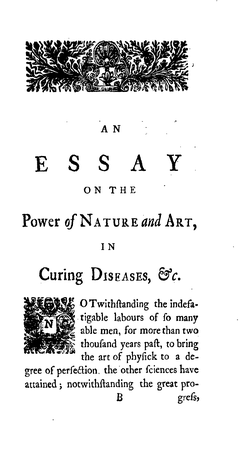
We required an algorithm that could ignore the text and draw bounding boxes around the two ornaments on the page. To solve this problem we enlisted Dirk Gorissen to develop a method using Python and OpenCV. I will not dive deeply into how Dirk’s algorithm works here. Basically it uses combines heuristics of where ornaments are typically located and how they look with various image filtering techniques to weed out text and other artifacts on the page to leave just the artwork intact.
Here is a demonstration of how each of the different stages of the algorithm work using on the single page shown above as an example:
Ornaments are visually very dense compared to the text. In the first stage the image is cleaned removing dust and stains in the white space of the page. Then through several iterations of blurring and contouring are applied until just the ornaments are left as single contours as seen in stage 5. A bounding box is then drawn around these contours and content of these boxes is then extracted from the original image.
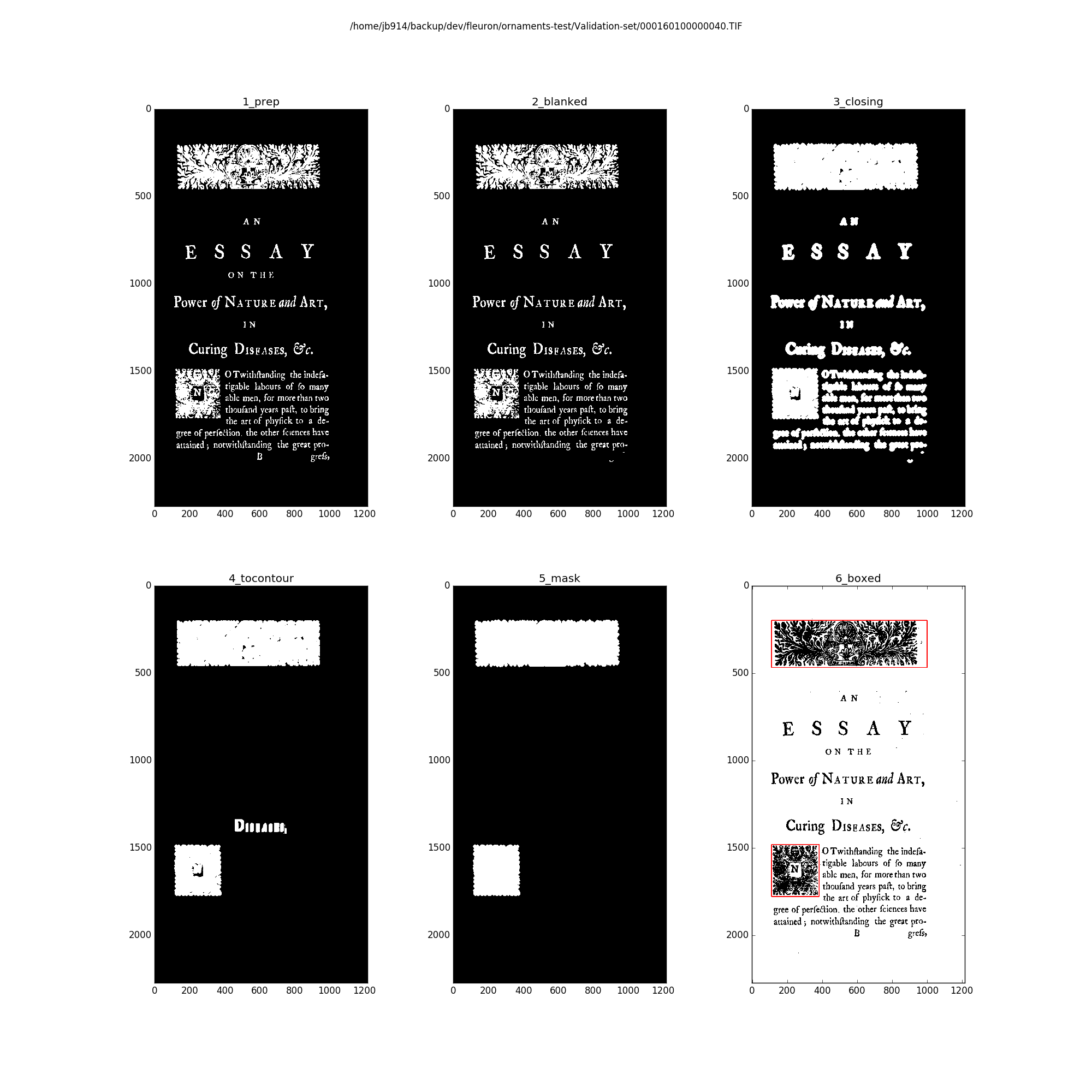
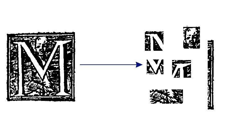
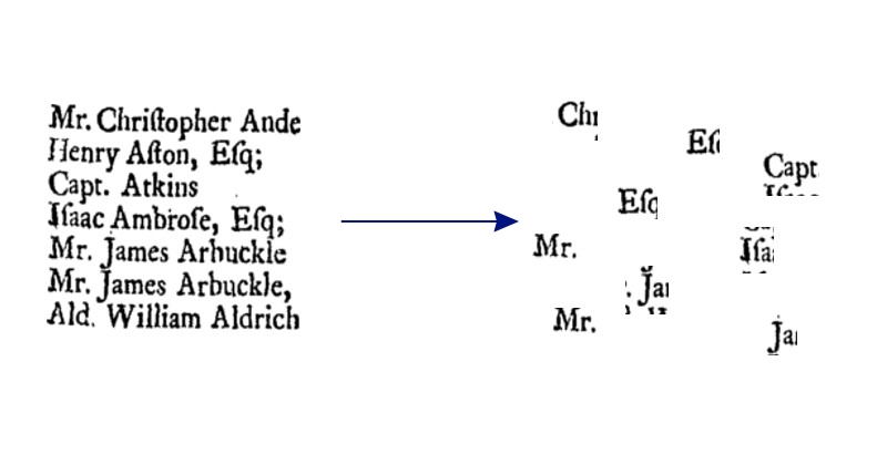
This method is simple and effective, but it is also apt to falsely classifying blocks of text. In the following example you can see clearly how this can happen:
After running extraction on all of the pages, I found that in a random sample of the images, most of them were just images of blocks of text! However, given that most of the pages in the dataset contain only text and no ornaments, perhaps this is to be expected even if the algorithm is fairly good at removing text.
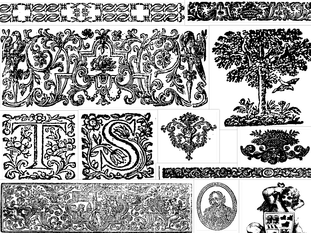
After extracting the ornaments from a large sample of the books, I hand labeled a random sample of 15000 images as valid and invalid. Here is a collage of valid images:
Here is a collage of invalid images that we want to filter out:
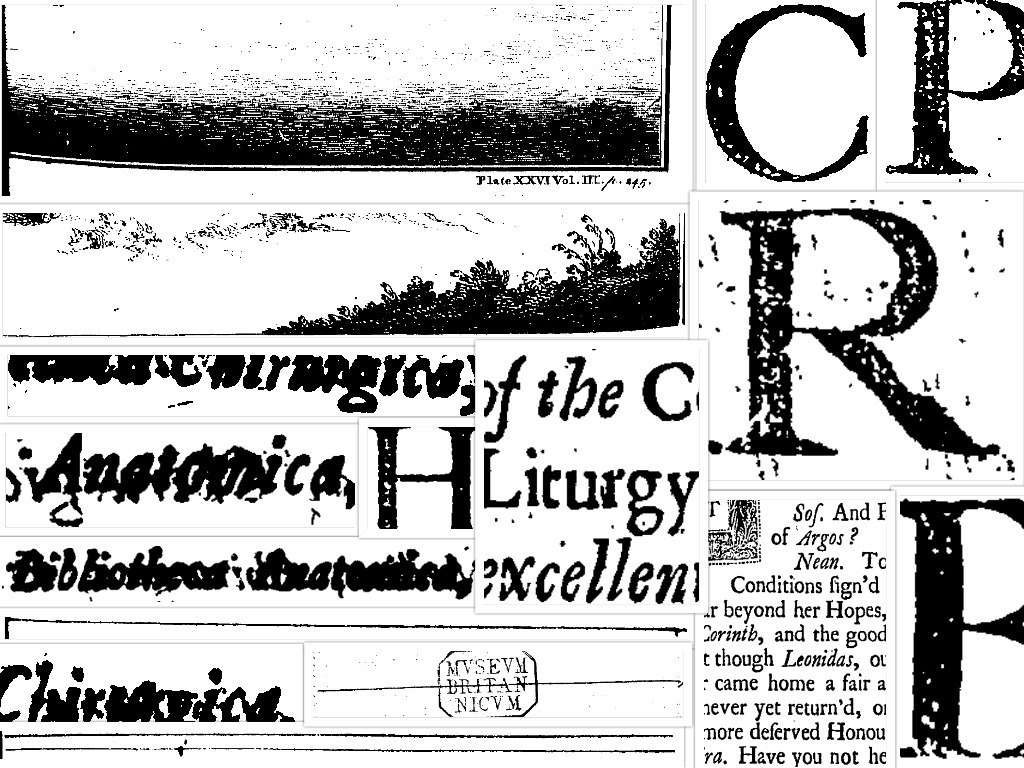
Image Filtering Pipeline
The choice of image representation is essential to getting a well performing machine learning based classifier. The Images are black and white and so we can’t use any colour features and contain very rich textures. The pipeline for the image filtering system:
- Create a labelled data set for training
- Represent each training image by a vector using Bag of Visual Words
- Train a classifier on the vector to discriminate between valid and invalid images
- Apply the classifier to unseen images in the data set.
Bag of Visual Words (BoVW)
The Bag of Visual Words (BoVW) method is a common feature representation of images in computer vision. The method is directly inspired by the Bag of Words (BoW) method used in text classificiation. In the BoW method, the basic idea is that a text document is split up into its component words. Each of the words in the document is then matched to a word in the dictionary, and the number of unique words in the document is counted. The text document is then represented as a sparse histogram of word counts that is as long as the dictionary.
This histogram can be interpreted as a vector in some high dimensional space, and two different documents will be represented by two different vectors. So for a dictionary with $D$ words the vector for document $i$ is:
\[v_i = [n(w_1,i), n(w_2,i), ..., n(w_D, i)]\]Where $n(w)$ counts the number of occurrences of word $w$. The distance between these two vectors (e.g. L2, cosine, etc) can therefore be used as a proxy for the similarity of the two documents. If everything is working well, then a low distance will indicate high similarity and a large distance will represent a high dissimilarity. With this representation we are able to throw machine learning algorithms at the data or do document retrieval.
BoVW is exactly the same method except that instead of using actual words it uses ‘visual words’ extracted from the images. Visual words basically take the form of ‘iconic’ patches or fragments of an image.
1. Extract notable features from the images
2. Learn a visual dictionary
Use a clustering algorithm like k-means with a apriori number of clusters (>1000) to learn a set of $k$ compound visual words.
3. Quantize features using the visual vocabulary
Now we could then take an image, find its visual words and match each of those words to their nearest equivalent in the dictionary.
4. Represent images by histogram of visual word counts
By counting how many times a word in the dictionary is matched, the image can be re-represented as a histogram of word counts:
Similar looking images will have contains many of the same words and counts.
SIFT - The Visual Word
Now that we have outlined the concept of the BoVW method, what do we actually use as the ‘visual word’? To create the visual words I used SIFT - ‘Scale Invariant Feature Transform’. SIFT is a method for detecting multiple interesting keypoints in a grey-scale image and describing each of those points using a 128 dimensional vector. The SIFT descriptor is invariant to scale, rotation, and illumination, which is why it is such a popular method in classification and CBIR. An excellent technical description of SIFT can be found here.
OpenCV has an implementation of a SIFT detector included. The following code finds all the keypoints in an image and draws them back onto the image.
img = cv2.imread('image_2.png')
img_gray = cv2.cvtColor(img, cv2.COLOR_BGR2GRAY)
kp, desc = sift.detectAndCompute(img_gray, None)
img2 = cv2.drawKeypoints(img_gray, kp, flags=cv2.DRAW_MATCHES_FLAGS_DRAW_RICH_KEYPOINTS)

cv2.imwrite('image_sift_2.png', img2)
Here is the output of this for two images from the dataset, one valid and the other invalid:


There is a simple improvement that can be made to SIFT called RootSIFT. RootSIFT is a small modification to the SIFT descriptor that corrects the L2 distance between two SIFT descriptors. This generally always improves performance for classification and image retrieval. Here is an implementation in python:
def rootsift_descriptor(f):
    """
    Extract root sift descriptors from image stored in file f
    :param: f : str or unicode filename
    :return: desc : numpy array [n_sift_desc, 128]
    """
    img = cv2.imread(f)
    img_gray = cv2.cvtColor(img, cv2.COLOR_BGR2GRAY)
    sift = cv2.SIFT()
    kp, desc = sift.detectAndCompute(img_gray, None)

    if desc is None:
        print('Warning: No SIFT features found in {}'.format(f))
        return None

    desc /= (desc.sum(axis=1, keepdims=True) + 1e-7)
    desc = np.sqrt(desc)

    return desc
Building a Visual Word Dictionary
To create a visual word dictionary we need to first collect and store all the RootSIFT descriptors from a large sample of images from our dataset. Here I used a sample size of 50,000 images. For 50,000 images, $N \approx 1~ billion$. The following script iterates through every image in the target directory, finds the RootSIFT descriptors of the image, and then stores them in a large $N\times128$ array in a HDF5 file.
import os
import glob
import cv2
import tables
import numpy as np
from bovw import rootsift_descriptor
from random import sample, shuffle


def create_descriptor_bag(filelist):
    """
    creates an array of descriptor vectors generated from every
    file in filelist
    """
    X = np.empty((0, 128), dtype=np.float32)
    N = len(filelist)
    for n, f in enumerate(filelist):
        print('Processing file: {} of {}...'.format(n, N))
        desc = rootsift_descriptor(f)
        if desc is not None:
            X = np.vstack((X, desc))
    return X


def main():
    h5f = tables.openFile('/scratch/ECCO/rootsift_vectors_50k.hdf', 'w')
    atom = tables.Atom.from_dtype(np.dtype('Float32'))
    ds = h5f.createEArray(h5f.root,
                          'descriptors',
                          atom,
                          shape=(0, 128),
                          expectedrows=1000000)

    PATH = '/home/jb914/ECCO_dict/random50k/'
    all_files = glob.glob(os.path.join(PATH, '*.png'))
    rand_sample = [all_files[i] for i in sample(range(1, len(all_files)), 5000)]
    chunk_size = 100
    for i in xrange(0,len(rand_sample), chunk_size):
        print('Creating rootsift descriptor bag...')
        X = create_descriptor_bag(rand_sample[i:i+chunk_size])
        print(X[0].shape)
        print(len(X))

        print('Writing file: rootsift_vectors_5000.hdf')
        for i in xrange(len(X)):
            ds.append(X[i][None])
        ds.flush()
    #ds[:] = X
    h5f.close()


if __name__ == '__main__':
    main()
HDF5 files are great for storing large multidimensional arrays of data to disk because they store the meta-data of the array dimensions and allow for streaming the data from disk to memory. This is especially useful when the full data is much larger than memory like here.
Creating the dictionary is the hardest and most time consuming part with BoVW. There are many vectors to cluster, the number of words is very large (between 1000 and 1,000,000), and the vectors are high dimensional. This stretches the capabilities of many clustering algorithms in all possible ways. In my experiments I found that the standard K-Means clustering algorithm quickly became intractable for larger numbers of vectors and clusters. Moreover the algorithm is offline - it needs to see all the data at once. Algorithms better suited for this task are approximate k-means (AKM) and mini-batch k-means.
I found success with two open source implementations of these in fastcluster (AKM), and in MiniBatchKMeans from scikit-learn. Fastcluster has the advantage that it uses distributed parallelism via MPI to split the large data up across multiple machines. However this useful code lacks documentation and no longer maintained. MiniBatchKMeans on the other hand isn’t parallel, however it does allow for streaming of the data through memory so it works great with HDF5.
In my experiments I found that setting the dictionary size to 20,000 words was sufficient.
The following script can stream a HDF5 file in a user defined number of chunks performing clustering with those chunks. The total clustering time for this was approximately 24 hours running in serial on a Intel Xeon Ivybridge CPU.
from __future__ import print_function
import numpy as np
import tables
import pickle
from sklearn.cluster import MiniBatchKMeans
from time import time


def main(n_clusters, chunk=0, n_chunks=32, checkpoint_file=None):
    datah5f = tables.open_file('/scratch/ECCO/rootsift_vectors_50k.hdf', 'r')
    shape = datah5f.root.descriptors.shape
    datah5f.close()

    print('Read in SIFT data with size in chunks: ', shape)
    print('Running MiniBatchKMeans with cluster sizes: ', n_clusters)

    c = n_clusters
    print('n_clusters:', c)

    if checkpoint_file:
        mbkm = pickle.load(open(checkpoint_file, 'r'))
    else:
        mbkm = MiniBatchKMeans(n_clusters=c, batch_size=10000,
                               init_size=30000, init='random',
                               compute_labels=False)

    step = shape[0] / n_chunks
    start_i = chunk*step
    for i in xrange(start_i, shape[0], step):
        datah5f = tables.open_file('/scratch/ECCO/rootsift_vectors_{}.hdf'.format(datasize), 'r')
        X = datah5f.root.descriptors[i:i+step]
        datah5f.close()

        t0 = time()
        mbkm.partial_fit(X)
        print('\t ({} of {}) Time taken: {}'.format(chunk, n_chunks, time()-t0))
        chunk += 1
        pickle.dump(mbkm, open('chkpt_{}.p'.format(n_clusters), 'w'))

    X = mbkm.cluster_centers_
    print(X.shape)
    f = tables.open_file('fleuron_codebook_{}.hdf'.format(n_clusters), 'w')
    atom = tables.Atom.from_dtype(X.dtype)
    ds = f.create_carray(f.root, 'clusters', atom, X.shape)
    ds[:] = X
    f.close()


if __name__ == '__main__':
    main(n_clusters=20000, chunk=0, n_chunks=4, checkpoint_file=None)
Matching Key Points to the Dictionary
With the dictionary created the next step is to represent all the images in the labeled training set as a histogram of matching keypoints. This is a nearest neighbour matching problem so with a brute force algorithm this is a $O(N)$ so this is slow for very high numbers of words. Faster nearest neighbour matching can be achieved with the FLANN library. OpenCV contains a wrapper for FLANN. I wrote a class that uses the FLANN matcher in OpenCV to match an array of descriptors to a codebook:
FLANN_INDEX_COMPOSITE = 3
FLANN_DIST_L2 = 1


class Codebook(object):
    def __init__(self, hdffile):
        clusterf = tables.open_file(hdffile)
        self._clusters = np.array(clusterf.get_node('/clusters'))
        clusterf.close()

        self._clusterids = np.array(xrange(0, self._clusters.shape[0]), dtype=np.int)
        self.n_clusters = self._clusters.shape[0]

        self._flann = cv2.flann_Index(self._clusters,
                                      dict(algorithm=FLANN_INDEX_COMPOSITE,
                                           distance=FLANN_DIST_L2,
                                           iterations=10,
                                           branching=16,
                                           trees=50))

    def predict(self, Xdesc):
        """
        Takes Xdesc a (n,m) numpy array of n img descriptors length m and returns
        (n,1) where every n has been assigned to a cluster id.
        """
        (_, m) = Xdesc.shape
        (_, cm) = self._clusters.shape
        assert m == cm

        result, dists = self._flann.knnSearch(Xdesc, 1, params={})
        return result
The following code takes a list of image files and a dictionary and returns the count vectors for each of those image files using the sparse matrix type from scipy. It is also multi-threaded using the joblib library:
def count_vector(f, codebook):
    """
    Takes a list of SIFT vectors from an image and matches
    each SIFT vector to its nearest equivalent in the codebook
    :param: f : Image file path
    :return: countvec : sparse vector of counts for each visual-word in the codebook
    """
    desc = rootsift_descriptor(f)
    if desc is None:
        # if no sift features found return 0 count vector
        return lil_matrix((1, codebook.n_clusters), dtype=np.int)

    matches = codebook.predict(desc)
    unique, counts = np.unique(matches, return_counts=True)

    countvec = lil_matrix((1, codebook.n_clusters), dtype=np.int)
    countvec[0, unique] = counts
    return countvec


class CountVectorizer(object):
    def __init__(self, vocabulary_file, n_jobs=1):
        self._codebook = Codebook(hdffile=vocabulary_file)
        if n_jobs == -1:
            self.n_jobs = cpu_count()
        else:
            self.n_jobs = n_jobs

    def transform(self, images):
        """
        Transform image files to a visual-word count matrix.
        :param: images : iterable
                    An iterable of str or unicode filenames
        :return: X : sparse matrix, [n_images, n_visual_words]
                     visual-word count matrix
        """

        sparse_rows = Parallel(backend='threading', n_jobs=self.n_jobs)(
            (delayed(count_vector)(f, self._codebook) for f in images)
        )

        X = lil_matrix((len(images), self._codebook.n_clusters),
                       dtype=np.int)

        for i, sparse_row in enumerate(sparse_rows):
            X[i] = sparse_row

        return X.tocsr()
Given a list of files the following code will return the count vectors for those images:
vectorizer = CountVectorizer('codebook_20k.hdf', n_jobs=-1)
Xcounts = vectorizer.transform(images)
tf-idf
Not all words are created equal, some are more frequent than others. This is the same in human language and in the create visual vocabulary. Words like ‘the’, ‘what’, ‘where’, etc will swamp the count vectors of english words in almost all english documents. Clearly they are less interesting than a rare word like ‘disestablishment’ and that we’d like two different documents both containing a word like ‘disestablishment’ to have a high similarity. So we’d like to reweight words which appear in few documents so that they have a higher importance, and words that appear in most documents to have lower importance. In another case, if a document only contained the word ‘disestablishment’ 1000 times should it be 1000 times more relevant than a document containing it once? So within an individual document we may want to reweight words that are repeated over and over so that they cannot artificially dominate.
These two reweightings can be achieved using tf-idf (term frequency inverse document frequency) weighting. This weighting is designed to reflect how important a particular word is in a document corpus. It is perfectly applicable in our visual word case also. Scikit-learn has an implementation of a tf-idf transformer for text classification that we can repurpose here. To following produces the final representation for the training data that we can use in the machine learning algorithm, $X$.
from sklearn.feature_extraction.text import TfidfTransformer
transformer = TfidfTransformer()
X = transformer.fit_transform(Xcount)
Visualisation of BoVW
That that we’ve transformed the images into tf-idf weighted, 20k dimensional, sparse vectors to visual word counts, we can visualise them and see if there is any apparent structure in this high dimensional data. Great algorithms for visualising high dimensional data are PCA and T-SNE, both of which have implementations in scikit-learn. I found here that PCA worked best. For high dimensional sparse data, the TruncatedSVD algorithm works best:
from sklearn.decomposition import TruncatedSVD

svd = TruncatedSVD(n_components=2)
Z = svd.fit_transform(X)
We can plot this with the images inlined and with colours representing the valid (red) and invalid (blue) labels:
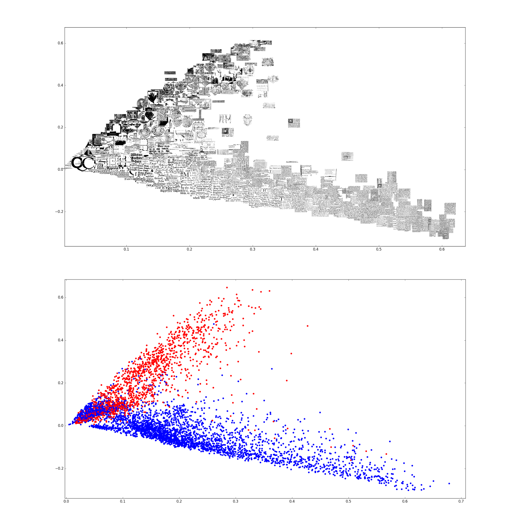
You can clearly see that there is clear structure in the higher dimensions and that the valid and invalid images separate quite well from each other. This is quite promising for the performance of a machine learning algorithm!
Classifying the Bad Images with Machine Learning
I tried a number of algorithms including Random forest, logistic regression and linear SVM. I found that SVM with a linear kernel by far performed the best compared to the other algorithms.
from sklearn.svm import LinearSVC

clf = LinearSVC()
clf.fit(X_train, y_train)
LinearSVC with the default settings performed very well with $97\%$ accuracy. High accuracy is generally a good sign, especially here where the numbers of valid and invalid images are of a similar size. Two other important statistics for classification are precision and recall.
Recall is a measure of what the probability that the classifier will identify and image as invalid given that it is invalid: $P(\hat{y}=1 | y=1)$. You can think of recall as the ratio of the number of images correctly classed as invalid to the number of all invalid images.
Precision on the other hand is a measure of the probability that an image is invalid given that the classifier says it is invalid: $P(y=1|\hat{y}=1)$. You can think of precision as the ratio of the number of images correctly classed as invalid to the number of all images classified.
The difference between them is subtle (here is a great explanation of the difference), but you may want to favour a trade-off of one for the other depending on your business case. In our case it is worse to misclassify a valid images as invalid because we are losing good images. We would much rather have some invalid images get through than lose good images, which is the same as favouring extra precision over recall.
We can tune the precision by adjusting the class weights of the Linear SVM, such that the penalty for classifying a valid image as invalid is much worse than classifying an invalid image as valid. I used cross-validation to find the best values for these. These give the valid images a weight of 20 and invalid images a weight of 0.1:
from sklearn.svm import LinearSVC

clf = LinearSVC(class_weight={0: 20, 1: 0.1})
clf.fit(X_train, y_train)
This yielded the final performance of $95\%$ accuracy, $99.5\%$ precision, and $93.8\%$ recall:
Confusion matrix:
 [[1134   11]
 [ 161 2439]]
Accuracy score:  0.954072096128
False Positive Rate:  0.00960698689956
False Negative Rate:  0.0619230769231
Precision:  0.995510204082
Recall:  0.938076923077
F1 Score:  0.965940594059
The performance of approach this is very good. The trained classifier was then applied across the whole image dataset. In the end there were approximately 3 million invalid images and 2 million valid images detected.
Further Ideas
Image search
The BoVW approach is also very useful for image retrieval. This means that given some image we can find duplications and similar looking images in the rest of the image set simply by finding the BoVW vectors that are closest to that image’s own BoVW vector. This is just a nearest neighbour search. It is complicated by the number of images because scaling nearest neighbour search with large numbers of vectors that don’t necessarily fit into memory relies on more complicated algorithms.
Neural Networks
Convolutional Neural Networks (CNNs) have shown great application in image classification in recent years. While they perform well at classification, they also have the advantage that they can discover vector representations of the images given the just the raw pixels. So it doesn’t require all this work with inventing a representation for images such as BoVW. The downside is that they require a lot of data (10s of thousands of examples) to be effective. Rather than hand labelling more examples, it would be quicker to look at the output of images classified by the SVM, and eyeball any false negatives or false positives in there. Artificial data could also be created using image transformations like rotation and inversion.